Image Recognition: Text Detection (Optical Character Recognition) using Google Cloud Vision API

Google Cloud Vision API helps in label detection, face detection, logo detection, landmark detection and text detection (OCR: Optical Character Recognition). In this article, we will see how can we use Google Cloud Vision API to extract the text from the image? This is a step by step guide for text detection (OCR) using Google Cloud Vision API. Let's follow it.

I will directly start from step 5. First 4 steps are same as mentioned in my previous post on label detection using Google Cloud Vision API.

You can download my Jupyter notebook containing below code from here.

 
Step 5: Import required libraries

from googleapiclient.discovery import build
from oauth2client.client import GoogleCredentials
from base64 import b64encode

You may get import error "no module name..." if you have not already installed Google API Python client. Use following command to install it.

pip install --upgrade google-api-python-client

If you also get import error for oauth2client, you must install it using following command:

pip3 install --upgrade oauth2client

Step 6: Load credentials file

Load the credentials file (which we created in step 3 of my previous article) and create a service object using it.

CREDENTIAL_FILE = 'credentials.json'
credentials = GoogleCredentials.from_stream(CREDENTIAL_FILE)
service = build('vision', 'v1', credentials=credentials)

Step 7: Load image file (from which we need to extract the text)

I will load an image of cover page of my deep learning book and encode it so that it becomes compatible with the cloud vision API.

IMAGE_FILE = book_cover_page.jpg'

with open(IMAGE_FILE, 'rb') as file:
    image_data = file.read()
    encoded_image_data = b64encode(image_data).decode('UTF-8')

Step 8: Create a batch request

We will create a batch request which we will send to the cloud vision API. In the batch request, we will include the above encoded image and the instruction as TEXT_DETECTION.

batch_request = [{
    'image':{'content':encoded_image_data},
    'features':[{'type':'TEXT_DETECTION'}],
}]

Step 9: Create a request

request = service.images().annotate(body={'requests':batch_request})

Step 10: Execute the request

response = request.execute()

This step will throw an error if you have not enabled billing (as mentioned in step 4 of my previous article). So, you must enable the billing in order to use Google Cloud Vision API. The charges are very reasonable. So, don't think too much and provide credit card details. For me, Google charged INR 1 and then refunded it back.

Step 11: Process the response

For error handling, include this code:

if 'error' in response:
    raise RuntimeError(response['error'])

We are interested in text annotations here. So, fetch it from the response and display the results.

labels = response['responses'][0]['textAnnotations']

extracted_text = extracted_texts[0]
print(extracted_text['description'], extracted_text['boundingPoly'])

Output:

Objective Type Questions and Answers in Deep Learning
Deep
Learning
ARTIFICIAL
INTELLIGENCE
MACHINE
LEARNING
DEEP
LEARNING
NARESH KUMAR
 {'vertices': [{'x': 42, 'y': 77}, {'x': 2365, 'y': 77}, {'x': 2365, 'y': 3523}, {'x': 42, 'y': 3523}]}

You can test the above code using different images and check the accuracy of the API.

Image Recognition: Label Detection using Google Cloud Vision API

Google Cloud Vision API helps in label detection, face detection, logo detection, landmark detection and text detection. In this article, we will see how can we use Google Cloud Vision API to identify labels in the image? This is a step by step guide for label detection using Google Cloud Vision API. Let's follow it.

Step 1: Setup a Google Cloud Account

A) Go to: https://console.cloud.google.com/
B) Login with your google credentials
C) You will see a dashboard. Create a Project if not already created.

Step 2: Enable Cloud Vision API

A) Go to console
B) Click on Navigation Menu
C) Click on API & Services >> Library
D) Search "cloud vision" and you will get the "Cloud Vision API". Enable this API if not already enabled.

Step 3: Download credentials file

A) Go to console
B) Click on Navigation Menu
C) Click on API & Services >> Credentials
D) Click on Create Credentials dropdown >> Service account key >> New service account
E) Enter Service account name
F) Select any role. I had selected Project >> Viewer
G) Save the file as JSON on your hard drive. Rename it to 'credentials.json'.

Step 4: Add billing information

A) Go to console
B) Click on Navigation Menu
C) Click on Billing

Now open the Jupyter notebook and try using this API. You can download my Jupyter notebook containing below code from here.
 
Step 5: Import required libraries

from googleapiclient.discovery import build
from oauth2client.client import GoogleCredentials
from base64 import b64encode

You may get import error "no module name..." if you have not already installed Google API Python client. Use following command to install it.

pip install --upgrade google-api-python-client

If you also get import error for oauth2client, you must install it using following command:

pip3 install --upgrade oauth2client

Step 6: Load credentials file

Load the credentials file (which we created in step 3) and create a service object using it.

CREDENTIAL_FILE = 'credentials.json'
credentials = GoogleCredentials.from_stream(CREDENTIAL_FILE)
service = build('vision', 'v1', credentials=credentials)

Step 7: Load image file (which needs to be tested)

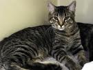
We will load an image of a cat and encode it so that it becomes compatible with the cloud vision API.

IMAGE_FILE = 'cat.jpg'
with open(IMAGE_FILE, 'rb') as file:
    image_data = file.read()
    encoded_image_data = b64encode(image_data).decode('UTF-8')

Step 8: Create a batch request

We will create a batch request which we will send to the cloud vision API. In the batch request, we will include the above encoded image and the instruction as LABEL_DETECTION.

batch_request = [{
    'image':{'content':encoded_image_data},
    'features':[{'type':'LABEL_DETECTION'}],
}]

Step 9: Create a request

request = service.images().annotate(body={'requests':batch_request})

Step 10: Execute the request

response = request.execute()

This step will throw an error if you have not enabled billing (as mentioned in step 4). So, you must enable the billing in order to use Google Cloud Vision API. The charges are very reasonable. So, don't think too much and provide credit card details. For me, Google charged INR 1 and then refunded it back.

Step 11: Process the response

For error handling, include this code:

if 'error' in response:
    raise RuntimeError(response['error'])

We are interested in label annotations here. So, fetch it from the response and display the results.

labels = response['responses'][0]['labelAnnotations']

for label in labels:
    print(label['description'], label['score'])

Output:

Cat 0.99598557
Mammal 0.9890478
Vertebrate 0.9851104
Small to medium-sized cats 0.978553
Felidae 0.96784574
European shorthair 0.960582
Tabby cat 0.9573447
Whiskers 0.9441685
Dragon li 0.93990624
Carnivore 0.9342105

You can test the above code using different images and check the accuracy of the API.

Image Recognition using Pre-trained VGG16 model in Keras

Lets use a pre-trained VGG16 model to predict an image from ImageNet database. We will load an image, convert that image to numpy array, preprocess that array and let the pre-trained VGG16 model predict the image.

VGG16 is a CNN model. To know more about CNN, you can visit my this post. We are not fine-tuning the VGG16 model here. We are using it as it is. To fine-tune the existing VGG16 model, you can visit my this post.

You can download my Jupyter notebook containing following code from here.

Step 1: Import required libraries

import numpy as np
from keras.applications import vgg16
from keras.preprocessing import image

Step 2: Load pre-trained weights from VGG16 model for ImageNet dataset

model = vgg16.VGG16(weights='imagenet')

Step 3: Load image to predict

img = image.load_img('cat.jpg', target_size=(224, 224))
img

Please note that we need to reshape the image to 224X224 as it is a requirement for VGG16 model. You can download this image from ImageNet official website.

Step 4: Convert the image into numpy array

arr = image.img_to_array(img)
arr.shape

(224, 224, 3)

Step 5: Expand the array dimension

arr = np.expand_dims(arr, axis=0)
arr.shape

(1, 224, 224, 3)

Step 6: Preprocess the array

arr = vgg16.preprocess_input(arr)
arr

Step 7: Predict from the model

predictions = model.predict(arr)

predictions

We get an array as an output which is hard to understand. So, lets simplify it and see top 5 predictions made by the VGG16 model.

vgg16.decode_predictions(predictions, top=5)

[[('n02123045', 'tabby', 0.7138179),
  ('n02123159', 'tiger_cat', 0.21695374),
  ('n02124075', 'Egyptian_cat', 0.043560617),
  ('n04040759', 'radiator', 0.0053847637),
  ('n04553703', 'washbasin', 0.0024860944)]]

So, as per VGG16 model prediction, the given image may be a tabby (71%) or a tiger cat (21%). You can try the same with different images from ImageNet database and check your results.

Solving a regression problem using a Sequential Neural Network Model in Keras

Lets solve a regression problem using neural networks. We will build a sequential model in Keras to predict house prices based on some parameters. We will use KerasRegressor to build a regression model.

You can download housing_data.csv from here. You can also download my Jupyter notebook containing below code of Neural Network Regression implementation.

Step 1: Import required libraries like pandas, numpy, sklearn, keras and matplotlib

import numpy as np
import pandas as pd

from sklearn.preprocessing import MinMaxScaler
from sklearn.model_selection import train_test_split
from sklearn.metrics import mean_absolute_error, mean_squared_error

from keras.models import Sequential
from keras.layers import Dense
from keras.wrappers.scikit_learn import KerasRegressor

import matplotlib.pyplot as plt
%matplotlib inline

Step 2: Load and examine the dataset

dataset = pd.read_csv('housing_data.csv')
dataset.head()
dataset.shape
dataset.describe(include='all')

Please note that "describe()" is used to display the statistical values of the data like mean and standard deviation.

Step 3: Mention X and Y axis

X=dataset.iloc[:,0:13]
y=dataset.iloc[:,13].values

X contains the list of attributes
Y contains the list of labels

Step 4: Split the dataset into training and testing dataset

X_train, X_test, y_train, y_test = train_test_split(X, y, test_size = 0.20, random_state=0) 

Step 5: Scale the features

scaler = MinMaxScaler()
X_train = scaler.fit_transform(X_train)
X_test = scaler.transform(X_test)
y = y.reshape(-1,1)
y = scaler.fit_transform(y)

This step is must for neural networks. Feature scaling is very important for neural networks to perform better and predict accurate results. We should scale both X and y data.

Step 6: Build a neural network

def build_regression_model():
    model = Sequential()
    model.add(Dense(50, input_dim=13, activation='relu'))
    model.add(Dense(50, activation='relu'))
    model.add(Dense(50, activation='relu'))
    model.add(Dense(1, activation='linear'))
    model.compile(optimizer='adam', loss='mean_squared_error')
    return model

We are creating a sequential model with fully connected layers. We are using four layers (one input layer, one output layer and two hidden layers). Input layer and hidden layers are using "relu" activation function while output layer is using "linear" activation function. 

Input layer and hidden layers contain 50 neurons and output layer contains only one neuron as we need to output only one value (predicted house price). You can change the number of neurons in the input and hidden layers as per your data and model performance. Number of hidden layers and number of neurons in each layer are the hyperparameters which you need to tune as the the performance of the model. 

We are using "adam" optimizer and mean square error as a loss function.

We can also use dropout in hidden layers for regularization. But, for this example, I am skipping this step for simplification.

Step 7: Train the neural network

regressor = KerasRegressor(build_fn=build_regression_model, batch_size=32, epochs=150) 
training_history = regressor.fit(X_train,y_train)

We are using 150 epochs with batch size of 32. Number of epochs and batch size are also the hyperparameters which need to be tuned. 

Step 8: Print a loss plot

plt.plot(training_history.history['loss'])
plt.show()

This plot shows that after around 140 epochs, the loss does not vary so much. That is why, I have taken number of epochs as 150 in step 7 while training the neural network.

Step 9: Predict from the neural network

y_pred= regressor.predict(X_test)
y_pred

The y_pred is a numpy array that contains all the predicted values for the input values in the X_test.

Lets see the difference between the actual and predicted values.

df=pd.DataFrame({'Actual':y_test, 'Predicted':y_pred})  
df 

Step 10: Check the accuracy

meanAbsoluteError = mean_absolute_error(y_test, y_pred)
meanSquaredError = mean_squared_error(y_test, y_pred)
rootMeanSquaredError = np.sqrt(meanSquaredError)
print('Mean Absolute Error:', meanAbsoluteError)  
print('Mean Squared Error:', meanSquaredError)  
print('Root Mean Squared Error:', rootMeanSquaredError)

Output:
Mean Absolute Error: 2.9524098807690193 Mean Squared Error: 19.836363961675836 Root Mean Squared Error: 4.453803314210882

We have got the root mean square error as 4.45. We can further decrease this error using cross validation and tuning our hyperparameters. I am leaving it for you to practice.

Step 11: Visualize the results using scatter plot 

plt.scatter(range(len(y_test)), y_test, c='g')
plt.scatter(range(len(y_test)), y_pred, c='b')
plt.xlabel('Test data')
plt.ylabel('Predicted data')
plt.show()

We are displaying test labels and predicted values in different colors (green and blue). From the scatter plot, we can visualize that our neural network has done a great job.

Step 12: Visualize results using regression plot

To further visualize the predicted results, we can draw a regression plot.

fig, ax = plt.subplots()
ax.scatter(y_test, y_pred)
ax.plot([y_test.min(), y_test.max()], [y_test.min(), y_test.max()], 'k--', lw=4)
ax.set_xlabel('Test data')
ax.set_ylabel('Predicted data')
plt.show()

I hope, I was able to demonstrate this regression problem to a large extent. If you have further any doubt, please post a comment.

Fine-tune VGG16 model for image classification in Keras

Keras framework provides us a lot of pre-trained general purpose deep learning models which we can fine-tune as per our requirements. We don't need to build a complex model from scratch. In my last article, we built a CNN model from scratch for image classification. Instead of that, we can just fine-tune an existing, well-trained, well-proven, widely accepted CNN model which will save our a lot of effort, time and money.

VGG16 is a proven proficient algorithm for image classification (1000 classes of images). Keras framework already contain this model. We will import this model and fine-tune it to classify the images of dogs and cats (only 2 classes instead of 1000 classes).

You can download my Jupyter notebook containing below code from here.

Step 1: Import the required libraries

import numpy as np
import matplotlib.pyplot as plt
%matplotlib inline

import keras
from keras.preprocessing.image import ImageDataGenerator
from keras.models import Sequential
from keras.layers import Dense
from keras.optimizers import Adam

from sklearn.metrics import confusion_matrix, accuracy_score, classification_report

Step 2: Create directory structure to contain images

We will create a directory structure which will contain the images of dogs and cats.

I have created a directory "cats_and_dogs". Under this directory, I have created 3 other directories "test", "train" and "valid". All these 3 directories contain "cat" and "dog" directories. 

1. "cat" and "dog" directories under "test" directory contain 5 images of cats and dogs respectively. Total 10 images for testing.

2. "cat" and "dog" directories under "train" directory contain 20 images of cats and dogs respectively. Total 40 images for training.

3. "cat" and "dog" directories under "valid" directory contain 8 images of cats and dogs respectively. Total 16 images for validation.

Step 3: Data Preparation

train_path = 'C:/cats_and_dogs/train'
valid_path = 'C:/cats_and_dogs/valid'
test_path = 'C:/cats_and_dogs/test'

train_batches = ImageDataGenerator().flow_from_directory(train_path, target_size=(224,224), classes=['dog','cat'], batch_size=10)

valid_batches = ImageDataGenerator().flow_from_directory(valid_path, target_size=(224,224), classes=['dog','cat'], batch_size=4)

test_batches = ImageDataGenerator().flow_from_directory(test_path, target_size=(224,224), classes=['dog','cat'], batch_size=10)

Output:
Found 40 images belonging to 2 classes. Found 16 images belonging to 2 classes. Found 10 images belonging to 2 classes.

In the above code, we are generating the images of 224x224 pixels and categorizing these images into cat and dog classes. It is clear from the output that we have 40 images for training, 16 images for validation and 10 images for testing as mentioned in step 2.

Step 4: Print the images

Lets output some of the images which we have prepared in step 3. Following is the standard code to print the images (copied from Keras documentation)

def plots(ims, figsize=(12,6), rows=1, interp=False, titles=None):
    if type(ims[0]) is np.ndarray:
        ims = np.array(ims).astype(np.uint8)
        if (ims.shape[-1] != 3):
            ims = ims.transpose((0,2,3,1))
    f = plt.figure(figsize=figsize)
    cols = len(ims)//rows if len(ims) % 2 == 0 else len(ims)//rows + 1
    for i in range(len(ims)):
        sp = f.add_subplot(rows, cols, i+1)
        sp.axis('Off')
        if titles is not None:
            sp.set_title(titles[i], fontsize=16)
        plt.imshow(ims[i], interpolation=None if interp else 'none')

Now, lets print the first batch of training images:

imgs, labels = next(train_batches)
plots(imgs, titles=labels)

Output:

We can see the scaled images of 10 cats and dogs. If you run again the above code, it will fetch next 10 images from training dataset as we are using batch size of 10 for training images.

Step 5: Load and analyze VGG16 model

vgg16_model = keras.applications.vgg16.VGG16()
vgg16_model.summary()
type(vgg16_model)

In the above code, first line will load the VGG16 model. It may take some time. By executing second line, we can see summary of the existing model. It has a lot of convolutional, pooling and dense layers. Executing third line, we can see this model is of type "Model". In next step, we will create a model of type "Sequential".

Step 6: Fine-tune VGG16 model

Following are the steps involved in fine-tuning a model:

1. Copy all the hidden layers in a new model
2. Remove output layer
3. Freeze the hidden layers
4. Add custom output layer

For more details on fine-tuning a model, please visit my this post.

Lets perform all the above steps.

model = Sequential() for layer in vgg16_model.layers[:-1]: model.add(layer)

In the above code, we have created a new sequential model and copied all the layers of VGG16 model except the last layer which is an output layer. We have done this because we want our custom output layer which will have only two nodes as our image classification problem has only two classes (cats and dogs).

Now, if we execute following statement, we will get replica of existing VGG16 model, except output layer.

model.summary()

Now, lets freeze the hidden layers as we don't want to change any weight and bias associated with these layers. We want to use these layers as it is as all these layers are already well trained on image classification problem.

for layer in model.layers: layer.trainable = False

Now, add a custom output layer with only two nodes and softmax as activation function.

model.add(Dense(2, activation='softmax'))
model.summary()

Now, our new fine-tuned model is ready. Lets train it with new data and then predict from it.

Step 7: Compile the model

model.compile(Adam(lr=0.0001), loss='categorical_crossentropy', metrics=['accuracy'])

Using Adam as an optimizer and categorical cross entropy as loss function.

Step 8: Train the model

model.fit_generator(train_batches, steps_per_epoch=4, validation_data=valid_batches, validation_steps=4, epochs=5, verbose=2)

Executing this step will take some time as we are using 5 epochs.

Step 9: Predict from the model

Lets print first batch of the test images.

test_imgs, test_labels = next(test_batches) plots(test_imgs, titles=test_labels)

From the output, we can see that it shows the final results in form of [0. 1.], [1. 0.] etc. Lets format this output so that we can get it in form of 0, 1 etc.

test_labels = test_labels[:,0] test_labels

Now, finally make prediction.

predictions = model.predict_generator(test_batches, steps=1, verbose=0)
predictions

It shows the predictions in form of probabilities. Lets round it off.

rounded_predictions = np.round(predictions[:,0])
rounded_predictions

Step 10: Check the accuracy

confusionMatrix = confusion_matrix(test_labels, rounded_predictions)
accuracyScore = accuracy_score(test_labels, rounded_predictions)
classificationReport = classification_report(test_labels, rounded_predictions)
print(confusionMatrix)
print(accuracyScore * 100)
print(classificationReport)

Please note that we won't get desired accuracy with this small dataset. We need thousands of image to train our model to get desired accuracy. We can use data augmentation to increase the data. You can download thousands of images of cats and dogs from Kaggle to train this model.