Thursday, July 5, 2012

Couchbase Architecture

After receiving a lot of good feedback and comment on my last blog on MongoDb, I was encouraged to do another deep dive on another popular document oriented db; Couchbase.

I have been a long-time fan CouchDb and has wrote a blog on it many years ago.  After it merges with Membase, I am very excited to take a deep look into it again.

Couchbase is the merge of two popular NOSQL technologies: 
  • Membase, which provides persistence, replication, sharding to the high performance memcached technology
  • CouchDB, which pioneers the document oriented model based on JSON
Like other NOSQL technologies, both Membase and CouchDB are built from the ground up on a highly distributed architecture, with data shard across machines in a cluster.  Built around the Memcached protocol, Membase provides an easy migration to existing Memcached users who want to add persistence, sharding and fault resilience on their familiar Memcached model.  On the other hand, CouchDB provides first class support for storing JSON documents as well as a simple RESTful API to access them.  Underneath, CouchDB also has a highly tuned storage engine that is optimized for both update transaction as well as query processing.  Taking the best of both technologies, Membase is well-positioned in the NOSQL marketplace.

Programming model

Couchbase provides client libraries for different programming languages such as Java / .NET / PHP / Ruby / C / Python / Node.js

For read, Couchbase provides a key-based lookup mechanism where the client is expected to provide the key, and only the server hosting the data (with that key) will be contacted.

Couchbase also provides a query mechanism to retrieve data where the client provides a query (for example, range based on some  secondary key) as well as the view (basically the index).  The query will be broadcasted to all servers in the cluster and the result will be merged and sent back to the client.

For write, Couchbase provides a key-based update mechanism where the client sends in an updated document with the key (as doc id).  When handling write request, the server will return to client’s write request as soon as the data is stored in RAM on the active server, which offers the lowest latency for write requests.

Following is the core API that Couchbase offers.  (in an abstract sense)

# Get a document by key

doc = get(key)

# Modify a document, notice the whole document 
#   need to be passed in

set(key, doc)

# Modify a document when no one has modified it 
#  since my last read

casVersion = doc.getCas()
cas(key, casVersion, changedDoc)

# Create a new document, with an expiration time 
#   after which the document will be deleted

addIfNotExist(key, doc, timeToLive)

# Delete a document

delete(key)

# When the value is an integer, increment the integer

increment(key)

# When the value is an integer, decrement the integer

decrement(key)

# When the value is an opaque byte array, append more 
#  data into existing value 

append(key, newData)

# Query the data 

results = query(viewName, queryParameters)

In Couchbase, document is the unit of manipulation.  Currently Couchbase doesn't support server-side execution of custom logic.  Couchbase server is basically a passive store and unlike other document oriented DB, Couchbase doesn't support field-level modification.  In case of modifying documents, client need to retrieve documents by its key, do the modification locally and then send back the whole (modified) document back to the server.  This design tradeoff network bandwidth (since more data will be transferred across the network) for CPU (now CPU load shift to client).

Couchbase currently doesn't support bulk modification based on a condition matching.  Modification happens only in a per document basis.  (client will save the modified document one at a time).

Transaction Model

Similar to many NOSQL databases, Couchbase’s transaction model is primitive as compared to RDBMS.  Atomicity is guaranteed at a single document and transactions that span update of multiple documents are unsupported.  To provide necessary isolation for concurrent access, Couchbase provides a CAS (compare and swap) mechanism which works as follows …
  • When the client retrieves a document, a CAS ID (equivalent to a revision number) is attached to it.
  • While the client is manipulating the retrieved document locally, another client may modify this document.  When this happens, the CAS ID of the document at the server will be incremented.
  • Now, when the original client submits its modification to the server, it can attach the original  CAS ID in its request.  The server will verify this ID with the actual ID in the server.  If they differ, the document has been updated in between and the server will not apply the update.
  • The original client will re-read the document (which now has a newer ID) and re-submit its modification. 
Couchbase also provides a locking mechanism for clients to coordinate their access to documents.  Clients can request a LOCK on the document it intends to modify, update the documents and then releases the LOCK.  To prevent a deadlock situation, each LOCK grant has a timeout so it will automatically be released after a period of time.

Deployment Architecture

 In a typical setting, a Couchbase DB resides in a server clusters involving multiple machines.  Client library will connect to the appropriate servers to access the data.  Each machine contains a number of daemon processes which provides data access as well as management functions.


The data server, written in C/C++, is responsible to handle get/set/delete request from client.  The Management server, written in Erlang, is responsible to handle the query traffic from client, as well as manage the configuration and communicate with other member nodes in the cluster.

Virtual Buckets

The basic unit of data storage in Couchbase DB is a JSON document (or primitive data type such as int and byte array) which is associated with a key.  The overall key space is partitioned into 1024 logical storage unit called "virtual buckets" (or vBucket).  vBucket are distributed across machines within the cluster via a map that is shared among servers in the cluster as well as the client library.


High availability is achieved through data replication at the vBucket level.  Currently Couchbase supports one active vBucket zero or more standby replicas hosted in other machines.  Curremtly the standby server are idle and not serving any client request.  In future version of Couchbase, the standby replica will be able to serve read request.

Load balancing in Couchbase is achieved as follows:
  • Keys are uniformly distributed based on the hash function
  • When machines are added and removed in the cluster.  The administrator can request a redistribution of vBucket so that data are evenly spread across physical machines.

Management Server

Management server performs the management function and co-ordinate the other nodes within the cluster.  It includes the following monitoring and administration functions

Heartbeat: A watchdog process periodically communicates with all member nodes within the same cluster to provide Couchbase Server health updates.

Process monitor: This subsystem monitors execution of the local data manager, restarting failed processes as required and provide status information to the heartbeat module.

Configuration manager: Each Couchbase Server node shares a cluster-wide configuration which contains the member nodes within the cluster, a vBucket map.  The configuration manager pull this config from other member nodes at bootup time.

Within a cluster, one node’s Management Server will be elected as the leader which performs the following cluster-wide management function
  • Controls the distribution of vBuckets among other nodes and initiate vBucket migration
  • Orchestrates the failover and update the configuration manager of member nodes
If the leader node crashes, a new leader will be elected from surviving members in the cluster.

When a machine in the cluster has crashed, the leader will detect that and notify member machines in the cluster that all vBuckets hosted in the crashed machine is dead.  After getting this signal, machines hosting the corresponding vBucket replica will set the vBucket status as “active”.  The vBucket/server map is updated and eventually propagated to the client lib.  Notice that at this moment, the replication level of the vBucket will be reduced.  Couchbase doesn’t automatically re-create new replicas which will cause data copying traffic.  Administrator can issue a command to explicitly initiate a data rebalancing.  The crashed machine, after reboot can rejoin the cluster.  At this moment, all the data it stores previously will be completely discard and the machine will be treated as a brand new empty machine.

As more machines are put into the cluster (for scaling out), vBucket should be redistributed to achieve a load balance.  This is currently triggered by an explicit command from the administrator.  Once receive the “rebalance” command, the leader will compute the new provisional map which has the balanced distribution of vBuckets and send this provisional map to all members of the cluster.

To compute the vBucket map and migration plan, the leader attempts the following objectives:
  • Evenly distribute the number of active vBuckets and replica vBuckets among member nodes.
  • Place the active copy and each replicas in physically separated nodes.
  • Spread the replica vBucket as wide as possible among other member nodes.
  • Minimize the amount of data migration
  • Orchestrate the steps of replica redistribution so no node or network will be overwhelmed by the replica migration.
Once the vBucket maps is determined, the leader will pass the redistribution map to each member in the cluster and coordinate the steps of vBucket migration.  The actual data transfer happens directly between the origination node to the destination node.

Notice that since we have generally more vBuckets than machines.  The workload of migration will be evenly distributed automatically.  For example, when new machines are added into the clusters, all existing machines will migrate some portion of its vBucket to the new machines.  There is no single bottleneck in the cluster.

Throughput the migration and redistribution of vBucket among servers, the life cycle of a vBucket in a server will be in one of the following states
  • “Active”:  means the server is hosting the vBucket is ready to handle both read and write request
  • “Replica”: means the server is hosting the a copy of the vBucket that may be slightly out of date but can take read request that can tolerate some degree of outdate.
  • “Pending”: means the server is hosting a copy that is in a critical transitional state.  The server cannot take either read or write request at this moment.
  • “Dead”: means the server is no longer responsible for the vBucket and will not take either read or write request anymore.

Data Server

Data server implements the memcached APIs such as get, set, delete, append, prepend, etc. It contains the following key datastructure:
  • One in-memory hashtable (key by doc id) for the corresponding vBucket hosted.  The hashtable acts as both a metadata for all documents as well as a cache for the document content.  Maintain the entry gives a quick way to detect whether the document exists on disk.
  • To support async write, there is a checkpoint linkedlist per vBucket holding the doc id of modified documents that hasn't been flushed to disk or replicated to the replica.

To handle a "GET" request
  • Data server routes the request to the corresponding ep-engine responsible for the vBucket.
  • The ep-engine will lookup the document id from the in-memory hastable.  If the document content is found in cache (stored in the value of the hashtable), it will be returned.  Otherwise, a background disk fetch task will be created and queued into the RO dispatcher queue.
  • The RO dispatcher then reads the value from the underlying storage engine and populates the corresponding entry in the vbucket hash table.
  • Finally, the notification thread notifies the disk fetch completion to the memcached pending connection, so that the memcached worker thread can revisit the engine to process a get request.
To handle a "SET" request,  a success response will be returned to the calling client once the updated document has been put into the in-memory hashtable with a write request put into the checkpoint buffer.  Later on the Flusher thread will pickup the outstanding write request from each checkpoint buffer, lookup the corresponding document content from the hashtable and write it out to the storage engine.

Of course, data can be lost if the server crashes before the data has been replicated to another server and/or persisted.  If the client requires a high data availability across different crashes, it can issue a subsequent observe() call which blocks on the condition  that the server persist data on disk, or the server has replicated the data to another server (and get its ACK).  Overall speaking, the client has various options to tradeoff data integrity with throughput.

Hashtable Management

To synchronize accesses to a vbucket hash table, each incoming thread needs to acquire a lock before accessing a key region of the hash table. There are multiple locks per vbucket hash table, each of which is responsible for controlling exclusive accesses to a certain ket region on that hash table. The number of regions of a hash table can grow dynamically as more documents are inserted into the hash table.

To control the memory size of the hashtable, Item pager thread will monitor the memory utilization of the hashtable.  Once a high watermark is reached, it will initiate an eviction process to remove certain document content from the hashtable.  Only entries that is not referenced by entries in the checkpoint buffer can be evicted because otherwise the outstanding update (which only exists in hashtable but not persisted) will be lost.

After eviction, the entry of the document still remains in the hashtable; only the document content of the document will be removed from memory but the metadata is still there.  The eviction process stops after reaching the low watermark.  The high / low water mark is determined by the bucket memory quota. By default, the high water mark is set to 75% of bucket quota, while the low water mark is set to 60% of bucket quota. These water marks can be configurable at runtime.

In CouchDb, every document is associated with an expiration time and will be deleted once it is expired.  Expiry pager is responsible for tracking and removing expired document from both the hashtable as well as the storage engine (by scheduling a delete operation).

Checkpoint Manager
Checkpoint manager is responsible to recycle the checkpoint buffer, which holds the outstanding update request, consumed by the two downstream processes, Flusher and TAP replicator.  When all the request in the checkpoint buffer has been  processed, the checkpoint buffer will be deleted and a new one will be created.

TAP Replicator
TAP replicator is responsible to handle vBucket migration as well as vBucket replication from active server to replica server.  It does this by propagating the latest modified document to the corresponding replica server.

At the time a replica vBucket is established, the entire vBucket need to be copied from the active server to the empty destination replica server as follows
  • The in-memory hashtable at the active server will be transferred to the replica server.  Notice that during this period, some data may be updated and therefore the data set transfered to the replica can be inconsistent (some are the latest and some are outdated).
  • Nevertheless, all updates happen after the start of transfer is tracked in the checkpoint buffer.
  • Therefore, after the in-memory hashtable transferred is completed, the TAP replicator can pickup those updates from the checkpoint buffer.  This ensures the latest versioned of changed documents are sent to the replica, and hence fix the inconsistency.
  • However the hashtable cache doesn’t contain all the document content.  Data also need to be read from the vBucket file and send to the replica.  Notice that during this period, update of vBucket will happen in active server.  However, since the file is appended only, subsequent data update won’t interfere the vBucket copying process.
After the replica server has caught up, subsequent update at the active server will be available at its checkpoint buffer which will be pickup by the TAP replicator and send to the replica server.

CouchDB Storage Structure

Data server defines an interface where different storage structure can be plugged-in.  Currently it supports both a SQLite DB as well as CouchDB.  Here we describe the details of CouchDb, which provides a super high performance storage mechanism underneath the Couchbase technology.

Under the CouchDB structure, there will be one file per vBucket.  Data are written to this file in an append-only manner, which enables Couchbase to do mostly sequential writes for update, and provide the most optimized access patterns for disk I/O.  This unique storage structure attributes to Couchbase’s fast on-disk performance for write-intensive applications.

The following diagram illustrate the storage model and how it is modified by 3 batch updates (notice that since updates are asynchronous, it is perform by "Flusher" thread in batches).


The Flusher thread works as follows:

1) Pick up all pending write request from the dirty queue and de-duplicate multiple update request to the same document.

2) Sort each request (by key) into corresponding vBucket and open the corresponding file

3) Append the following into the vBucket file (in the following contiguous sequence)
  • All document contents in such write request batch.  Each document will be written as [length, crc, content] one after one sequentially.
  • The index that stores the mapping from document id to the document’s position on disk (called the BTree by-id)
  • The index that stores the mapping from update sequence number to the document’s position on disk.  (called the BTree by-seq)
The by-id index plays an important role for looking up the document by its id.  It is organized as a B-Tree where each node contains a key range.  To lookup a document by id, we just need to start from the header (which is the end of the file), transfer to the root BTree node of the by-id index, and then further traverse to the leaf BTree node that contains the pointer to the actual document position on disk.

During the write, the similar mechanism is used to trace back to the corresponding BTree node that contains the id of the modified documents.  Notice that in the append-only model, update is not happening in-place, instead we located the existing location and copy it over by appending.  In other words, the modified BTree node will be need to be copied over and modified and finally paste to the end of file, and then its parent need to be modified to point to the new location, which triggers the parents to be copied over and paste to the end of file.  Same happens to its parents’ parent and eventually all the way to the root node of the BTree.  The disk seek can be at the O(logN) complexity.

The by-seq index is used to keep track of the update sequence of lived documents and is used for asynchronous catchup purposes.  When a document is created, modified or deleted, a sequence number is added to the by-seq btree and the previous seq node will be deleted.  Therefore, for cross-site replication, view index update and compaction, we can quickly locate all the lived documents in the order of their update sequence.   When a vBucket replicator asks for the list of update since a particular time, it provides the last sequence number in previous update, the system will then scan through the by-seq BTree node to locate all the document that has sequence number larger than that, which effectively includes all the document that has been modified since the last replication.

As time goes by, certain data becomes garbage (see the grey-out region above) and become unreachable in the file.  Therefore, we need a garbage collection mechanism to clean up the garbage.  To trigger this process, the by-id and by-seq B-Tree node will keep track of the data size of lived documents (those that is not garbage) under its substree.  Therefore, by examining the root BTree node, we can determine the size of all lived documents within the vBucket.  When the ratio of actual size and vBucket file size fall below a certain threshold, a compaction process will be triggered  whose job is to open the vBucket file and copy the survived data to another file.

Technically, the compaction process opens the file and read the by-seq BTree at the end of the file.  It traces the Btree all the way to the leaf node and copy the corresponding document content to the new file.  The compaction process happens while the vBucket is being updated.  However, since the file is appended only, new changes are recorded after the BTree root that the compaction has opened, so subsequent data update won’t interfere with the compaction process.  When the compaction is completed, the system need to copy over the data that was appended since the beginning of the compaction to the new file.

View Index Structure

Unlike most indexing structure which provide a pointer from the search attribute back to the document.  The CouchDb index (called View Index) is better perceived as a denormalized table with arbitrary keys and values loosely associated to the document.

Such denormalized table is defined by a user-provided map() and reduce() function.

map = function(doc) {
   …
   emit(k1, v1)
   …
   emit(k2, v2)
   …
}

reduce = function(keys, values, isRereduce) {
    if (isRereduce) {
        // Do the re-reduce only on values (keys will be null)
    } else {
        // Do the reduce on keys and values
    }
    // result must be ready for input values to re-reduce

    return result
}

Whenever a document is created, updated, deleted, the corresponding map(doc) function will be invoked (in an asynchronous manner) to generate a set of key/value pairs.  Such key/value will be stored in a B-Tree structure.  All the key/values pairs of each B-Tree node will be passed into the reduce() function, which compute an aggregated value within that B-Tree node.  Re-reduce also happens in non-leaf B-Tree nodes which further aggregate the aggregated value of child B-Tree nodes.

The management server maintains the view index and persisted it to a separate file.

Create a view index is perform by broadcast the index creation request to all machines in the cluster.  The management process of each machine will read its active vBucket file and feed each surviving document to the Map function.  The key/value pairs emitted by the Map function will be stored in a separated BTree index file.  When writing out the BTree node, the reduce() function will be called with the list of all values in the tree node.  Its return result represent a partially reduced value is attached to the BTree node.

The view index will be updated incrementally as documents are subsequently getting into the system.  Periodically, the management process will open the vBucket file and scan all documents since the last sequence number.  For each changed document since the last sync, it invokes the corresponding map function to determine the corresponding key/value into the BTree node.  The BTree node will be split if appropriate.

Underlying, Couchbase use a back index to keep track of the document with the keys that it previously emitted.  Later when the document is deleted, it can look up the back index to determine what those key are and remove them.  In case the document is updated, the back index can also be examined; semantically a modification is equivalent to a delete followed by an insert.

The following diagram illustrates how the view index file will be incrementally updated via the append-only mechanism.


Query Processing

Query in Couchbase is made against the view index.  A query is composed of the view name, a start key and end key.  If the reduce() function isn’t defined, the query result will be the list of values sorted by the keys within the key range.  In case the reduce() function is defined, the query result will be a single aggregated value of all keys within the key range.


If the view has no reduce() function defined, the query processing proceeds as follows:
  • Client issue a query (with view, start/end key) to the management process of any server (unlike a key based lookup, there is no need to locate a specific server).
  • The management process will broadcast the request to other management process on all servers (include itself) within the cluster.
  • Each management process (after receiving the broadcast request) do a local search for value within the key range by traversing the BTree node of its view file, and start sending back the result (automatically sorted by the key) to the initial server.
  • The initial server will merge the sorted result and stream them back to the client.
 However, if the view has reduce() function defined, the query processing will involve computing a single aggregated value as follows:
  • Client issue a query (with view, start/end key) to the management process of any server (unlike a key based lookup, there is no need to locate a specific server).
  • The management process will broadcast the request to other management process on all servers (include itself) within the cluster.
  • Each management process do a local reduce for value within the key range by traversing the BTree node of its view file to compute the reduce value of the key range.  If the key range span across a BTree node, the pre-computed of the sub-range can be used.  This way, the reduce function can reuse a lot of partially reduced values and doesn’t need to recomputed every value of the key range from scratch.
  • The original server will do a final re-reduce() in all the return value from each other servers, and then passed back the final reduced value to the client.
To illustrate the re-reduce concept, lets say the query has its key range from A to F.


Instead of calling reduce([A,B,C,D,E,F]), the system recognize the BTree node that contains [B,C,D] has been pre-reduced and the result P is stored in the BTree node, so it only need to call reduce(A,P,E,F).

Update View Index as vBucket migrates
Since the view index is synchronized with the vBuckets in the same server, when the vBucket has migrated to a different server, the view index is no longer correct; those key/value that belong to a migrated vBucket should be discarded and the reduce value cannot be used anymore.

To keep track of the vBucket and key in the view index, each bTree node has a 1024-bitmask indicating all the vBuckets that is covered in the subtree (ie: it contains a key emitted from a document belonging to the vBucket).  Such bit-mask is maintained whenever the bTree node is updated.

At the server-level, a global bitmask is used to indicate all the vBuckets that this server is responsible for.

In processing the query of the map-only view, before the key/value pair is returned, an extra check will be perform for each key/value pair to make sure its associated vBucket is what this server is responsible for.

When processing the query of a view that has a reduce() function, we cannot use the pre-computed reduce value if the bTree node contains a vBucket that the server is not responsible for.  In this case, the bTree node’s bit mask is compared with the global bit mask.  In case if they are not aligned, then the reduce value need to be recomputed.


Here is an example to illustrate this process


Couchbase is one of the popular NOSQL technology built on a solid technology foundation designed for high performance.  In this post, we have examined a number of such key features:
  • Load balancing between servers inside a cluster that can grow and shrink according to workload conditions.  Data migration can be used to re-achieve workload balance.
  • Asynchronous write provides lowest possible latency to client as it returns once the data is store in memory.
  • Append-only update model pushes most update transaction into sequential disk access, hence provide extremely high throughput for write intensive applications.
  • Automatic compaction ensures the data lay out on disk are kept optimized all the time.
  • Map function can be used to pre-compute view index to enable query access.  Summary data can be pre-aggregated using the reduce function.  Overall, this cut down the workload of query processing dramatically.

For a review on NOSQL architecture in general and some theoretical foundation, I have wrote a NOSQL design pattern blog, as well as some fundamental difference between SQL and NOSQL.

For other NOSQL technologies, please read my other blog on MongoDb, Cassandra and HBase, Memcached

Special thanks to Damien Katz and Frank Weigel from Couchbase team who provide a lot of implementation details of Couchbase.

Monday, June 11, 2012

Predictive Analytics: Evaluate Model Performance

In previous posts, we have discussed various machine learning techniques including linear regression with regularization, SVM, Neural network, Nearest neighbor, Naive Bayes, Decision Tree and Ensemble models.  How do we pick which model is the best ?  or even whether the model we pick is better than a random guess ?  In this posts, we will cover how we evaluate the performance of the model and what can we do next to improve the performance.

Best guess with no model 

First of all, we need to understand the goal of our evaluation.  Are we trying to pick the best model ?  Are we trying to quantify the improvement of each model ?  Regardless of our goal, I found it is always useful to think about what the baseline should be.  Usually the baseline is what is your best guess if you don't have a model.

For classification problem, one approach is to do a random guess (with uniform probability) but a better approach is to guess the output class that has the largest proportion in the training samples.  For regression problem, the best guess will be the mean of output of training samples.

Prepare data for evaluation

In a typical setting, the set of data is divided into 3 disjoint groups; 20% data is set aside as testing data to evaluate the model we've trained.  The remaining 80% of data is dividing into k partitions.  k-1 partitions will be used as training data to train a model with a particular parameter value setting and 1 partition will be used as cross-validation data to pick the best parameter value that minimize the error of the cross-validation data.

As a concrete example, lets say we have 100 records available.  We'll set aside 20% which is 20 records for testing purposes and use the remaining 80 records to train the model.  Lets say the model has some tunable parameters (e.g. k in KNN, λ in linear model regularization).  For each particular parameter value, we'll conduct 10 rounds of training (ie: k = 10).  Within each round, we randomly select 90% which is 72 records to train a model and compute the error of prediction against the 8 unselected records.  Then we take the average error of these 10 rounds and pick the optimal parameter value that gives the minimal average error.  After picking the optimal tuning parameter,  we retrain the model using the whole 80 records.

To evaluate the predictive performance of the model, we'll test it against the 20 testing records we set aside at the beginning.  The details will be described below.

Measuring Regression Performance

For regression problem, measuring the distance between the estimated output from the actual output is used to quantify the model's performance.  Three measures are commonly used:  Root Mean Square Error, Relative Square Error and Coefficient of Determination.  Typically root mean square is used for measuring the absolute quantity of accuracy.


Mean Square Error MSE = (1/N) * ∑(yest – yactual)2
Root Mean Square Error RMSE = (MSE)1/2

To measure the accuracy with respect to the baseline, we use the ratio of MSE


Relative Square Error RSE = MSE / MSEbaseline
RSE = ∑(yest – yactual)2 / ∑(ymean – yactual)2

Coefficient Of Determination (also called R square) measures the variance that is explained by the model, which is the reduction of variance when using the model.  R square ranges from 0 to 1 while the model has strong predictive power when it is close to 1 and is not explaining anything when it is close to 0.

R2 = (MSEbaseline – MSE) / MSEbaseline
R2 = 1 – RSE

Here are some R code to compute these measures

> 
> Prestige_clean <- Prestige[!is.na(Prestige$type),]
> model <- lm(prestige~., data=Prestige_clean)
> score <- predict(model, newdata=Prestige_clean)
> actual <- Prestige_clean$prestige
> rmse <- (mean((score - actual)^2))^0.5
> rmse
[1] 6.780719
> mu <- mean(actual)
> rse <- mean((score - actual)^2) / mean((mu - actual)^2) 
> rse
[1] 0.1589543
> rsquare <- 1 - rse
> rsquare
[1] 0.8410457
> 

The Mean Square Error penalize the bigger difference more because of the square effect.  On the other hand, if we want to reduce the penalty of bigger difference, we can log transform the numeric quantity first.

Mean Square Log Error MSLE = (1/N) * ∑(log(y)est – log(y)actual)2
Root Mean Square Log Error RMSLE = (MSLE)1/2

Measuring Classification Performance

For classification problem, there are a couple of measures.
  • TP = Predict +ve when Actual +ve
  • TN = Predict -ve when Actual -ve
  • FP = Predict +ve when Actual -ve
  • FN = Predict -ve when Actual +ve
Precision = TP / Predict +ve = TP / (TP + FP)
Recall or Sensitivity = TP / Actual +ve = TP / (TP + FN)
Specificity = TN / Actual -ve = TN / (FP + TN)
Accuracy = (TP + TN) / (TP + TN + FP + FN)

Accuracy alone is not sufficient to represent the quality of prediction because the cost of making a FP may be different from the cost of making a FN.  F measures provides a tunable assigned weight for computing a final score and is commonly used to measure the quality of a classification model.

1/Fmeasure = α/recall + (1-α)/precision

Notice that most classification model is based on estimating a numeric score for each output class.  By choosing the cutoff point of this score, we can control the tradeoff between precision and recall.  We can plot the relationship between precision and recall at various cutoff points as follows ...

> library(ROCR)
> library(e1071)
> nb_model <- naiveBayes(Species~., data=iristrain)
> nb_prediction <- predict(nb_model,
                           iristest[,-5], 
                           type='raw') 
> score <- nb_prediction[, c("virginica")]
> actual_class <- iristest$Species == 'virginica'
> # Mix some noise to the score
> # Make the score less precise for illustration
> score <- (score + runif(length(score))) / 2
> pred <- prediction(score, actual_class)
> perf <- performance(pred, "prec", "rec")
> plot(perf)
> 


Another common plot is the ROC curve which plot the "sensitivity" (true positive rate) against 1 - "specificity" (false positive rate).  The area under curve "auc" is used to compare the quality between different models with varying cutoff points.  Here is how we produce the ROC curve.

> library(ROCR)
> library(e1071)
> nb_model <- naiveBayes(Species~., 
                         data=iristrain)
> nb_prediction <- predict(nb_model, 
                           iristest[,-5], 
                           type='raw') 
> score <- nb_prediction[, c("virginica")]
> actual_class <- iristest$Species == 'virginica'
> # Mix some noise to the score
> # Make the score less precise for illustration
> score <- (score + runif(length(score))) / 2
> pred <- prediction(score, actual_class)
> perf <- performance(pred, "tpr", "fpr")
> auc <- performance(pred, "auc")
> auc <- unlist(slot(auc, "y.values"))
> plot(perf)
> legend(0.6,0.3,c(c(paste('AUC is', auc)),"\n"),
         border="white",cex=1.0,
         box.col = "white")
> 


We can also assign the relative cost of making a false +ve and false -ve decision to find the best cutoff threshold.  Here is how we plot the cost curve

> # Plot the cost curve to find the best cutoff
> # Assign the cost for False +ve and False -ve
> perf <- performance(pred, "cost", cost.fp=4, cost.fn=1)
> plot(perf)
> 

From the curve, the best cutoff point 0.6 is where the cost is minimal.

Source of error: Bias and Variance

In model-based machine learning, we are making assumption that the underlying data follows some underlying mathematical model and during the training we try to fit the training data into this assumed model and determine the best model parameters which gives the minimal error.

One source of error is when our assumed model is fundamentally wrong (e.g. if the output has a non-linear relationship with the input but we are assuming a linear model).  This is known as the High Bias problem which we use an over-simplified model to represent the underlying data.

Another source of error is when the model parameters fits too specifically to the training data and not generalizing well to the underlying data pattern.  This is known as the High Variance problem and usually happen when there is insufficient training data compare to the number of model parameters.

High bias problem has the symptom that both training and cross-validation shows a high error rate and both error rate drops as the model complexity increases.  While the training error keep decreasing as the model complexity increases, the cross-validation error will increase after certain model complexity and this indicates the beginning of a high variance problem.  When the size of training data is fixed and the only thing we can choose is the model complexity, then we should choose the model complexity at the point where the cross-validation error is minimal.


Will getting more data help ?

When collecting more data cost both time and money, we need to carefully assess the situation before we spend our effort to do so.  There is a very pragmatic technique suggested by Andrew Ng from Stanford by plotting the error against the size of data.  In this approach, we sample different size of training data to train up different models and plot both the cross-validation error and the training error with respect to the training sample size.
If the problem is a high-bias problem, the error curve will look like the following.

In this case, collecting more data would not help.  We should spend our effort to do the following instead.
  • Add more input features by talking to domain experts to identify more input signals and collect them.
  • Add more input features by combining existing input features in a non-linear way.
  • Try more complex, machine learning models. (e.g. increase the number of hidden layers in Neural Network, or increase the number of Neurons at each layer)
If the problem is a high-variance problem because we over-estimate the model complexity, then we should reduce the model complexity by throwing away attributes that has low influence to the output.  We don't have to gather more data.

The only situation where having more data will be helpful is when the underlying data model is in fact complex.  Therefore we cannot just reduce the complexity as this will immediately results in a high-bias problem.  In this case, the error curve will have the following shape.


And the only way is to collect more training data such that overfitting is less likely to happen.

Evaluate the performance of a model is very important in the overall cycle of predictive analytics.  Hopefully this introductory post gives a basic idea on how this can be done.

Wednesday, June 6, 2012

Predictive Analytics: Decision Tree and Ensembles

Continue from my last post of walking down the list of machine learning technique.  In this post, I will covered Decision Tree and Ensemble methods.  We'll continue using the iris data we prepare in this earlier post.

Decision Tree

Decision Tree model is one of the oldest machine learning model and is usually used to illustrate the very basic idea of machine learning.  Based on a tree of decision nodes, the learning approach is to recursively divide the training data into buckets of homogeneous members through the most discriminative dividing criteria.  The measurement of "homogeneity" is based on the output label; when it is a numeric value, the measurement will be the variance of the bucket; when it is a category, the measurement will be the entropy or gini index of the bucket..


During the training, various dividing criteria based on the input will be tried (using in a greedy manner); when the input is a category (Mon, Tue, Wed ...), it will first be turned into binary (isMon, isTue, isWed ...) and then use the true/false as a decision boundary to evaluate the homogeneity; when the input is a numeric or ordinal value, the lessThan, greaterThan at each training data input value will be used as the decision boundary.

The training process stops when there is no significant gain in homogeneity by further split the Tree. The members of the bucket represented at leaf node will vote for the prediction; majority wins when the output is a category and member’s average is taken when the output is a numeric.

Here is an example in R

> install.packages('rpart')
> library(rpart)
> #Train the decision tree
> treemodel <- rpart(Species~., data=iristrain)
> plot(treemodel)
> text(treemodel, use.n=T)
> #Predict using the decision tree
> prediction <- predict(treemodel, newdata=iristest, type='class')
> #Use contingency table to see how accurate it is
> table(prediction, iristest$Species)
prediction   setosa versicolor virginica
  setosa         10          0         0
  versicolor      0         10         3
  virginica       0          0         7


Here is the decision tree that we have learned.

The good part of Tree is that it can take different data type of input and output variables which can be categorical, binary and numeric value.  It can handle missing attributes and outliers well.  The decision tree is also good in explaining reasoning for its prediction and therefore gives good insight about the underlying data.

The limitation of decision tree is that each decision boundary at each split point is a concrete binary decision. Also the decision criteria only consider one input attributes at a time but not a combination of multiple input variables. Another weakness of Tree is that once learned it cannot be updated incrementally. When new training data arrives, you have to throw away the old tree and retrain every data from scratch.  In practice, standalone decision tree and rarely used in practice as its predictive accuracy and relatively low.  Tree ensembles (described below) are the common way to use decision trees.

Tree Ensembles

Instead of picking a single model, Ensemble Method combines multiple models in a certain way to fit the training data.  There are two primary ways: “bagging” and “boosting”.  In “bagging”, we take a subset of training data (pick n random sample out of N training data with replacement) to train up each model.  After multiple models are trained, we use a voting scheme to predict future data.

“Boosting” is another approach in Ensemble Method.  Instead of sampling the input features, it samples the training data records, but it puts more emphasis on the training data that is wrongly predicted in previous iterations.  Initially each training data is equally weighted.  At each iteration, the data that is wrongly classified will have its weight increased. The final prediction will be voted by each tree learned at each iteration weighted by the accuracy of that tree.

Random Forest

Random Forest is one of the most popular bagging models; in additional to selecting n training data out of N, at each decision node of the tree, it randomly selects m input features from the total M input features (m ~ M^0.5) and learns a decision tree from it.  Finally each tree in the forest vote for the result.

Here is the R code to use Random Forest.

> install.packages(‘randomForest')
> library(randomForest)
> #Train 100 trees, random selected attributes
> model <- randomForest(Species~., data=iristrain, nTree=500)
> #Predict using the forest
> prediction <- predict(model, newdata=iristest, type='class')
> table(prediction, iristest$Species)
> importance(model)
             MeanDecreaseGini
Sepal.Length         7.807602
Sepal.Width          1.677239
Petal.Length        31.145822
Petal.Width         38.617223


Gradient Boosted Trees

Gradient Boosting Method is one of the most popular boosting methods. It is based on incrementally add a function that fits the gradient of a lost function of residuals
  1. Set i = 0 at the beginning, repeat until converge
  2. Learn a function F(X) to predict Y.  Basically find F that minimize expected(L(F(X) – Y)), where L is the lost function of the residual
  3. Learning another function g(X) to predict the gradient of above function
  4. Update F = F + a.g(X), where a is the learning rate
 Gradient Boosted Tree using decision tree as the learning model F.

Here is the sample code in R.

> library(gbm)
> iris2 <- iris
> newcol = data.frame(isVersicolor=(iris2$Species=='versicolor'))
> iris2 <- cbind(iris2, newcol)
> iris2[45:55,]
   Sepal.Length Sepal.Width Petal.Length Petal.Width    Species isVersicolor
45          5.1         3.8          1.9         0.4     setosa        FALSE
46          4.8         3.0          1.4         0.3     setosa        FALSE
47          5.1         3.8          1.6         0.2     setosa        FALSE
48          4.6         3.2          1.4         0.2     setosa        FALSE
49          5.3         3.7          1.5         0.2     setosa        FALSE
50          5.0         3.3          1.4         0.2     setosa        FALSE
51          7.0         3.2          4.7         1.4 versicolor         TRUE
52          6.4         3.2          4.5         1.5 versicolor         TRUE
53          6.9         3.1          4.9         1.5 versicolor         TRUE
54          5.5         2.3          4.0         1.3 versicolor         TRUE
55          6.5         2.8          4.6         1.5 versicolor         TRUE
> formula <- isVersicolor ~ Sepal.Length 
                              + Sepal.Width
                              + Petal.Length
                              + Petal.Width
> model <- gbm(formula, data=iris2, 
               n.trees=1000, 
               interaction.depth=2,
               distribution="bernoulli")
Iter   TrainDeviance   ValidDeviance   StepSize   Improve
     1        1.2714         -1.#IND     0.0010    0.0008
     2        1.2705         -1.#IND     0.0010    0.0004
     3        1.2688         -1.#IND     0.0010    0.0007
     4        1.2671         -1.#IND     0.0010    0.0008
     5        1.2655         -1.#IND     0.0010    0.0008
     6        1.2639         -1.#IND     0.0010    0.0007
     7        1.2621         -1.#IND     0.0010    0.0008
     8        1.2614         -1.#IND     0.0010    0.0003
     9        1.2597         -1.#IND     0.0010    0.0008
    10        1.2580         -1.#IND     0.0010    0.0008
   100        1.1295         -1.#IND     0.0010    0.0008
   200        1.0090         -1.#IND     0.0010    0.0005
   300        0.9089         -1.#IND     0.0010    0.0005
   400        0.8241         -1.#IND     0.0010    0.0004
   500        0.7513         -1.#IND     0.0010    0.0004
   600        0.6853         -1.#IND     0.0010    0.0003
   700        0.6266         -1.#IND     0.0010    0.0003
   800        0.5755         -1.#IND     0.0010    0.0002
   900        0.5302         -1.#IND     0.0010    0.0002
  1000        0.4901         -1.#IND     0.0010    0.0002

> prediction <- predict.gbm(model, iris2[45:55,], 
                            type="response", 
                            n.trees=1000)
> round(prediction, 3)
 [1] 0.127 0.131 0.127 0.127 0.127 0.127 0.687 0.688 
     0.572 0.734 0.722
> summary(model)
           var       rel.inf
1 Petal.Length 61.4203761582
2  Petal.Width 34.7557511871
3  Sepal.Width  3.5407662531
4 Sepal.Length  0.2831064016
>


GBM R package also gave the relative importance of the input features.
I have gone through most of the common machine learning techniques.  In this next post, I will covered how to evaluate the performance of these models in their predictive power.

Friday, June 1, 2012

Predictive Analytics: NeuralNet, Bayesian, SVM, KNN

Continuing from my previous blog in walking down the list of Machine Learning techniques.  In this post, we'll be covering Neural Network, Support Vector Machine, Naive Bayes and Nearest Neighbor.  Again, we'll be using the same iris data set that we prepared in the last blog.

Neural Network

Neural Network emulates how the human brain works by having a network of neurons that are interconnected and sending stimulating signal to each other.

In the Neural Network model, each neuron is equivalent to a logistic regression unit.  Neurons are organized in multiple layers where every neuron at layer i connects out to every neuron at layer i+1 and nothing else.


The tuning parameters in Neural network includes the number of hidden layers, number of neurons in each layer, as well as the learning rate.

There are no fixed rules to set these parameters and depends a lot in the problem domain.  My default choice is to use a single hidden layer and set the number of neurons to be the same as the input variables. The number of neurons at the output layer depends on how many binary outputs need to be learned.  In a classification problem, this is typically the number of possible values at the output category.

The learning happens via an iterative feedback mechanism where the error of training data output is used to adjusted the corresponding weights of input.  This adjustment will be propagated back to previous layers and the learning algorithm is known as back-propagation.

Here is an example in R

> library(neuralnet)
> nnet_iristrain <-iristrain
> #Binarize the categorical output
> nnet_iristrain <- cbind(nnet_iristrain, 
                          iristrain$Species == 'setosa')
> nnet_iristrain <- cbind(nnet_iristrain,
                          iristrain$Species == 'versicolor')
> nnet_iristrain <- cbind(nnet_iristrain, 
                          iristrain$Species == 'virginica')
> names(nnet_iristrain)[6] <- 'setosa'
> names(nnet_iristrain)[7] <- 'versicolor'
> names(nnet_iristrain)[8] <- 'virginica'
> nn <- neuralnet(setosa+versicolor+virginica ~ 
                  Sepal.Length+Sepal.Width
                              +Petal.Length
                              +Petal.Width,
                  data=nnet_iristrain, 
                  hidden=c(3))
> plot(nn)
> mypredict <- compute(nn, iristest[-5])$net.result
> # Put multiple binary output to categorical output
> maxidx <- function(arr) {
      return(which(arr == max(arr)))
  }
> idx <- apply(mypredict, c(1), maxidx)
> prediction <- c('setosa', 'versicolor', 'virginica')[idx]
> table(prediction, iristest$Species)
            
prediction   setosa versicolor virginica
  setosa         10          0         0
  versicolor      0         10         3
  virginica       0          0         7


Here is the plot of the Neural network we learn
Neural network is very good at learning non-linear function and also multiple outputs can be learnt at the same time.  However, the training time is relatively long and it is also susceptible to local minimum traps.  This can be mitigated by doing multiple rounds and pick the best learned model.

Support Vector Machine

Support Vector Machine provides a binary classification mechanism based on finding a dividing hyperplane between a set of samples with +ve and -ve outputs.  It assumes the data is linearly separable.

The problem can be structured as a quadratic programming optimization problem as maximizing the margin subjected to a set of linear constraints (ie: data output on one side of the line must be +ve while the other side is -ve).  This can be solved by quadratic programming technique.


If the data is not linearly separable due to noise (majority is still linearly separable), then an error term will be added to penalize the optimization.


If the data distribution is fundamentally non-linear, the trick is to transform the data to a higher dimension and hopefully the data is linearly separable in that higher dimension.  The optimization term turns out to be a dot product of the transformed points in the high dimensional space, which was found to be equivalent to perform a kernal function in the original (before transformation) space.


The kernal function provides a cheap way to equivalently transform the original point to a high dimension (since we don’t actually transform it) and perform the quadratic optimization in that high dimension space.

There are a couple tuning parameters (like the penalty / cost) and so the usual way is to do it in 2 steps, find the optimal parameter and then train the SVM model using that.  Here is the example code in R.

> library(e1071)
> tune <- tune.svm(Species~., 
                   data=iristrain, 
                   gamma=10^(-6:-1), 
                   cost=10^(1:4))
> summary(tune)
Parameter tuning of ‘svm’:
- sampling method: 10-fold cross validation 
- best parameters:
 gamma  cost
 0.001 10000
- best performance: 0.03333333 
> model <- svm(Species~., 
               data=iristrain, 
               method="C-classification", 
               kernel="radial", 
               probability=T, 
               gamma=0.001, 
               cost=10000)
> prediction <- predict(model, iristest)
> table(iristest$Species, prediction)
            prediction
             setosa versicolor virginica
  setosa         10          0         0
  versicolor      0         10         0
  virginica       0          3         7
>


SVM with Kernal function is a highly effective model and works well across a wide range of problem sets.  Although it is a binary classifier, it can be easily extended to multi-class classification by training a group of binary classifiers and using “one vs all” or “one vs one” to predict.

SVM predicts the output based on the distance to the dividing hyperplane, which doesn’t directly provide a probability estimation of its prediction.  Calibration technique can be used which basically learn a logistic regression model between the distance of the hyperplane and the binary output and using the logistic regression to estimate the probability.

SVM is a very powerful technique and perform good in a wide range of non-linear classification problems.  It works best when you have a small set of input features because it will expand the features into higher dimension space, providing that you also have a good size of training data (otherwise, overfit can happen).  However, SVM is not very scalable in dealing with large number (billions) of training data, so in that case, Logistic Regression with manually expanded feature set will be more pragmatic. 

Naive Bayes

From a probabilistic viewpoint, the predictive problem can be viewed as a conditional probability estimation; trying to find Y where P(Y | X) is maximized.

From Bayesian rule, P(Y | X) == P(X | Y) * P(Y) / P(X)

This is equivalent to finding Y where P(X | Y) * P(Y) is maximized.

Lets say input X contains 3 categorical features, X1, X2, X3.  In the general case, we assume each variable can potentially influence any other variable and therefore the joint distribution becomes:
P(X | Y) = P(X1 | Y) * P(X2 | X1, Y) * P(X3 | X1, X2, Y)

Notice the last term of the above equation has number of entries exponentially proportional to the number of input variables.


To reduce the complexity, we can make some independence assumption based on domain knowledge and remove some edges.  We form a Bayesian Network where the arrows indicate causal relationship.


In Naïve Bayes model, we take our independence assumption even further and assume each input variable are independent of each other given Y.


Since P(X | Y) == P(X1 | Y) * P(X2 | Y) * P(X3 | Y).
The problem is to find Y to maximize P(X1 | Y) * P(X2 | Y) * P(X3 | Y) * P(Y)

Each term can be learned by counting the training data.  Therefore we can estimate P(Y | X) and pick Y that maximize its value.

It is possible that some patterns never show up in training data ie: P(X1=a | Y=y) is 0.  To deal with this situation, we apply the smoothing technique by assuming we have seen the data of each possible value one more than actual.  Now ...

P(X1=a | Y=y) == (count(a, y) + 1) / (count(y) + m)
where m is the number of possible values in X1.

When the input features are numeric, say a = 2.75, we can assume X1 is normal distribution.  Find out the mean and standard deviation of X1 and then estimate P(X1=a) using the normal distribution function.

Here is how we use Naïve Bayes in R
> library(e1071)
> # Can handle both categorical and numeric input, 
> # but output must be categorical
> model <- naiveBayes(Species~., data=iristrain)
> prediction <- predict(model, iristest[,-5])
> table(prediction, iristest[,5])
            
prediction   setosa versicolor virginica
  setosa         10          0         0
  versicolor      0         10         2
  virginica       0          0         8
 

Notice the independence assumption is not true in most cases, nevertheless the system still perform incredibly well.  One strength of Naïve Bayes is it is highly scalable and can learn incrementally because all we do is to count the observed variables and update the probability distribution.

K Nearest Neighbor

K Nearest neighbor is also called instance-based learning, in contrast to model-based learning, because it is not learning any model at all.  The training process is basically memorizing all the training data.  To predict a new data point, we found the closest K (a tunable parameter) neighbors from the training set and let them vote for the final prediction.

To determine the “nearest neighbors”, a distance function need to be defined (e.g. Euclidean distance is a common one for numeric input variables).  The voting can also be weighted among the K-neighbors based on their distance from the new data point.


Here is the R code of using K-nearest neighbor for classification.

> library(class)
> train_input <- as.matrix(iristrain[,-5])
> train_output <- as.vector(iristrain[,5])
> test_input <- as.matrix(iristest[,-5])
> prediction <- knn(train_input, test_input, 
                    train_output, k=5)
> table(prediction, iristest$Species)
            
prediction   setosa versicolor virginica
  setosa         10          0         0
  versicolor      0         10         1
  virginica       0          0         9
> 


The strength of K nearest neighbor is its simplicity as no model needs to be trained. Incremental learning is automatic when more data arrives (and old data can be deleted as well). The weakness of KNN is it doesn't handle high number of dimensions well.

In my next post, I will finish up the other machine learning techniques on decision trees and ensemble methods.

Tuesday, May 29, 2012

Predictive Analytics: Generalized Linear Regression

In the previous 2 posts, we have covered how to visualize input data to explore strong signals as well as how to prepare input data to a form that is situation for learning.  In this and subsequent posts, I'll go through various machine learning techniques to build our predictive model.
  1. Linear regression
  2. Logistic regression
  3. Linear and Logistic regression with regularization
  4. Neural network
  5. Support Vector Machine
  6. Naive Bayes
  7. Nearest Neighbor
  8. Decision Tree
  9. Random Forest
  10. Gradient Boosted Trees
There are two general types of problems that we are interested in this discussion; Classification is about predicting a category (value that is discrete, finite with no ordering implied) while Regression is about predicting a numeric quantity (value is continuous, infinite with ordering).

For classification problem, we use the "iris" data set and predict its "species" from its "width" and "length" measures of sepals and petals.  Here is how we setup our training and testing data.

> summary(iris)
  Sepal.Length       Sepal.Width        Petal.Length    Petal.Width      
 Min.   :4.300000   Min.   :2.000000   Min.   :1.000   Min.   :0.100000  
 1st Qu.:5.100000   1st Qu.:2.800000   1st Qu.:1.600   1st Qu.:0.300000  
 Median :5.800000   Median :3.000000   Median :4.350   Median :1.300000  
 Mean   :5.843333   Mean   :3.057333   Mean   :3.758   Mean   :1.199333  
 3rd Qu.:6.400000   3rd Qu.:3.300000   3rd Qu.:5.100   3rd Qu.:1.800000  
 Max.   :7.900000   Max.   :4.400000   Max.   :6.900   Max.   :2.500000  
       Species  
 setosa    :50  
 versicolor:50  
 virginica :50  
                
> head(iris)
  Sepal.Length Sepal.Width Petal.Length Petal.Width Species
1          5.1         3.5          1.4         0.2  setosa
2          4.9         3.0          1.4         0.2  setosa
3          4.7         3.2          1.3         0.2  setosa
4          4.6         3.1          1.5         0.2  setosa
5          5.0         3.6          1.4         0.2  setosa
6          5.4         3.9          1.7         0.4  setosa
> 
# Prepare training and testing data
> testidx <- which(1:length(iris[,1])%%5 == 0)
> iristrain <- iris[-testidx,]
> iristest <- iris[testidx,]


For regression problem, we use the "Prestige" data set (imported from the "car" R package) and predict the degree of "prestige" from a set of input variables such as "income", "education", "job types" ... etc.  Here is how we setup our training and testing data.

> library(car)
> summary(Prestige)
   education            income              women         
 Min.   : 6.38000   Min.   :  611.000   Min.   : 0.00000  
 1st Qu.: 8.44500   1st Qu.: 4106.000   1st Qu.: 3.59250  
 Median :10.54000   Median : 5930.500   Median :13.60000  
 Mean   :10.73804   Mean   : 6797.902   Mean   :28.97902  
 3rd Qu.:12.64750   3rd Qu.: 8187.250   3rd Qu.:52.20250  
 Max.   :15.97000   Max.   :25879.000   Max.   :97.51000  
    prestige            census           type   
 Min.   :14.80000   Min.   :1113.000   bc  :44  
 1st Qu.:35.22500   1st Qu.:3120.500   prof:31  
 Median :43.60000   Median :5135.000   wc  :23  
 Mean   :46.83333   Mean   :5401.775   NA's: 4  
 3rd Qu.:59.27500   3rd Qu.:8312.500            
 Max.   :87.20000   Max.   :9517.000            
> head(Prestige)
                    education income women prestige census type
gov.administrators      13.11  12351 11.16     68.8   1113 prof
general.managers        12.26  25879  4.02     69.1   1130 prof
accountants             12.77   9271 15.70     63.4   1171 prof
purchasing.officers     11.42   8865  9.11     56.8   1175 prof
chemists                14.62   8403 11.68     73.5   2111 prof
physicists              15.64  11030  5.13     77.6   2113 prof
> testidx <- which(1:nrow(Prestige)%%4==0)
> prestige_train <- Prestige[-testidx,]
> prestige_test <- Prestige[testidx,]


To measure the performance of our prediction, here we use some simple metrics to get through this basic ideas.  For regression problem, we'll use the correlation between our prediction and the testing result.  For classification problem, we'll use the contingency table to measure the count of true/false positive/negative in our prediction.

Now we have set the stage, lets get started.

Linear Regression

Linear regression has the longest history in statistics, well understood and is the most popular machine learning model.  It is based on the assumption of a linear relationship exist between the input x1, x2 ... and output variable y (numeric).

y = Ɵ0 + Ɵ1x1 + Ɵ2x2 + …


The learning algorithm will learn the set of parameter such that the objective function: sum of square error ∑(yactual - yestimate)2 is minimized.

Here is the code examples in R.

> model <- lm(prestige~., data=prestige_train)
> summary(model)
Call:
lm(formula = prestige ~ ., data = prestige_train)

Residuals:
        Min          1Q      Median          3Q         Max 
-13.9078951  -5.0335742   0.3158978   5.3830764  17.8851752 

Coefficients:
                  Estimate     Std. Error  t value     Pr(>|t|)    
(Intercept) -20.7073113585  11.4213272697 -1.81304    0.0743733 .  
education     4.2010288017   0.8290800388  5.06710 0.0000034862 ***
income        0.0011503739   0.0003510866  3.27661    0.0016769 ** 
women         0.0363017610   0.0400627159  0.90612    0.3681668    
census        0.0018644881   0.0009913473  1.88076    0.0644172 .  
typeprof     11.3129416488   7.3932217287  1.53018    0.1307520    
typewc        1.9873305448   4.9579992452  0.40083    0.6898376    
---
Signif. codes:  0 ‘***’ 0.001 ‘**’ 0.01 ‘*’ 0.05 ‘.’ 0.1 ‘ ’ 1 

Residual standard error: 7.41604 on 66 degrees of freedom
  (4 observations deleted due to missingness)
Multiple R-squared: 0.820444,   Adjusted R-squared: 0.8041207 
F-statistic: 50.26222 on 6 and 66 DF,  p-value: < 0.00000000000000022204 

> # Use the model to predict the output of test data
> prediction <- predict(model, newdata=prestige_test)
> # Check for the correlation with actual result
> cor(prediction, prestige_test$prestige)
[1] 0.9376719009


The coefficient column gives an estimation of Ɵi, there is an associated p-value that gives the confidence of each estimated Ɵi.  For example, features not marked with at least one * can be safely ignored.

In the above model, education and income has a high influence to the prestige.

Linear regression has certain assumption about the underlying distribution of data which we need to validate.  This include the residuals (error) has normal distribution with a zero mean and constant variation.

> # verify if the residuals are normally distributed
> rs <- residuals(model)
> qqnorm(rs)
> qqline(rs)
> shapiro.test(rs)
        Shapiro-Wilk normality test
data:  rs 
W = 0.9744, p-value = 0.1424


Here is the plot of how the residual aligned with the normal distribution.

Logistic Regression

Logistic Regression is basically applying a transformation of the output of a linear regression such that it fits into the value of 0 to 1, and hence mimic the probability of a binary output.  Logistic regression is the most popular machine learning technique applied in solving classification problem.

In a classification problem, the output is binary rather than numeric, we can imagine of doing a linear regression and then compress the numeric output into a 0..1 range using the logit function
1/(1+e-t)

y = 1/(1 + e -(Ɵ0 + Ɵ1x1 + Ɵ2x2 + …))    


The objective function in logistic regression is different.  It is minimizing the entropy as follows ...
∑ (yactual * log yestimate + (1 - yactual) * log(1 - yestimate))

Here is the example R code to classify iris data.

> newcol = data.frame(isSetosa=(iristrain$Species == 'setosa'))
> traindata <- cbind(iristrain, newcol)
> head(traindata)
  Sepal.Length Sepal.Width Petal.Length Petal.Width Species isSetosa
1          5.1         3.5          1.4         0.2  setosa     TRUE
2          4.9         3.0          1.4         0.2  setosa     TRUE
3          4.7         3.2          1.3         0.2  setosa     TRUE
4          4.6         3.1          1.5         0.2  setosa     TRUE
6          5.4         3.9          1.7         0.4  setosa     TRUE
7          4.6         3.4          1.4         0.3  setosa     TRUE
> formula <- isSetosa ~ Sepal.Length + Sepal.Width
                        + Petal.Length + Petal.Width
> logisticModel <- glm(formula, data=traindata, 
                       family="binomial")
> # Predict the probability for test data
> prob <- predict(logisticModel, newdata=iristest, type='response')
> round(prob, 3)
  5  10  15  20  25  30  35  40  45  50  55  60  65  70  75 
  1   1   1   1   1   1   1   1   1   1   0   0   0   0   0 
 80  85  90  95 100 105 110 115 120 125 130 135 140 145 150 
  0   0   0   0   0   0   0   0   0   0   0   0   0   0   0 

Regression with Regularization

Notice our assumption of linearity between input and output variable above is not necessary true.  One technique is to combine existing features by multiplying them together and hope we are lucky enough to hit some useful combination.  Therefore we may end up having a large set of input features in our machine learning.

When we have a large size of input variable but moderate size of training data, we are subjected to the overfitting problem, which is our model fits too specific to the training data and not generalized enough for the data we haven't seen.  Regularization is the technique of preventing the model to fit too specifically to the training data.

In linear regression, it is found that overfitting happens when Ɵ has a large value.  So we can add a penalty that is proportional to the magnitude of Ɵ.  In L2 regularization (also known as Ridge regression), Σ square(Ɵi) will be added to the cost function, while In L1 regularization (also known as Lasso regression), Σ ||Ɵi|| will be added to the cost function.

Both L1, L2 will shrink the magnitude of Ɵi, L2 tends to make dependent input variables having the same coefficient while L tends to pick of the coefficient of variable to be non-zero and other zero.  In other words, L1 regression will penalize the coefficient of redundant variables that are linearly dependent and is frequently used to remove redundant features.

Combining L1 and L2, the general form of cost function becomes
Cost == Non-regularization-cost + λ (α.Σ ||Ɵi|| + (1- α).Σ square(Ɵi))

Notice there are 2 tunable parameters, lambda λ and alpha α.  Lambda controls the degree of regularization (0 means no-regularization, infinity means ignoring all input variables because all coefficients of them will be zero).  Alpha controls the degree of mix between L1 and L2. (0 means pure L2 and 1 means pure L1).

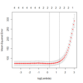
Glmnet is a popular regularization package.  The alpha parameter need to be supplied based on the application need (for selecting a reduced set of variables, alpha=1 is preferred).  The library provides a cross-validation test to automatically figure out what is the better lambda value.

Lets repeat the linear regression "prestige" data set and use regularization this time, we pick alpha = 0.7 to favor L1 regularization.

> library(glmnet)
> cv.fit <- cv.glmnet(as.matrix(prestige_train[,c(-4, -6)]), 
                      as.vector(prestige_train[,4]), 
                      nlambda=100, alpha=0.7, 
                      family="gaussian")
> plot(cv.fit)
> coef(cv.fit)
5 x 1 sparse Matrix of class "dgCMatrix"
                          1
(Intercept) 6.3876684930151
education   3.2111461944976
income      0.0009473793366
women       0.0000000000000
census      0.0000000000000
> prediction <- predict(cv.fit, 
                        newx=as.matrix(prestige_test[,c(-4, -6)]))
> cor(prediction, as.vector(prestige_test[,4]))
          [,1]
1 0.9291181193


Here is the cross-validation plot, which shows the best lambda with minimal mean square error.


Also we can repeat the logistic regression "iris" data set and use regularization this time, we pick alpha = 0.8 to even favor L1 regularization more.

> library(glmnet)
> cv.fit <- cv.glmnet(as.matrix(iristrain[,-5]), 
                      iristrain[,5], alpha=0.8, 
                      family="multinomial")
> prediction <- predict(cv.fit, 
                        newx=as.matrix(iristest[,-5]),
                        type="class")
> table(prediction, iristest$Species)
prediction   setosa versicolor virginica
  setosa         10          0         0
  versicolor      0         10         2
  virginica       0          0         8


Instead of picking lambda (the degree of regularization) based on cross validation, we can also based on the number of input variables that we want to retain.  So we can plot the "regularization path" which shows how the coefficient of each input variables changes when the lambda changes and pick the right lambda that filter out the number of input variables for us.

> # try alpha = 0, Ridge regression
> fit <- glmnet(as.matrix(iristrain[,-5]), 
                iristrain[,5], alpha=0, 
                family="multinomial")
> plot(fit)
> # try alpha = 0.8, Elastic net
> fit <- glmnet(as.matrix(iristrain[,-5]), 
                iristrain[,5], alpha=0.8, 
                family="multinomial")
> plot(fit)
> # try alpha = 1, Lasso regression
> fit <- glmnet(as.matrix(iristrain[,-5]), 
                iristrain[,5], alpha=1, 
                family="multinomial")
> plot(fit)


Here is the output of these plots.  Notice that as Alpha is closer to 1 (L1 regularization), it tends to have a stronger filter to the number of input variables.

In my next post, I will cover the other machine learning techniques.

Thursday, May 17, 2012

Predictive Analytics: Data Preparation

As a continuation of my last post on predictive analytics, in this post I will focus in describing how to prepare data for the training the predictive model., I will cover how to perform necessary sampling to ensure the training data is representative and fit into the machine processing capacity.  Then we validate the input data and perform necessary cleanup on format error, fill-in missing values and finally transform the collected data into our defined set of input features.

Different machine learning model will have its unique requirement in its input and output data type.  Therefore, we may need to perform additional transformation to fit the model requirement

Sample the data

If the amount of raw data is huge, processing all of them may require an extensive amount of processing power which may not be practical.  In this case it is quite common to sample the input data to reduce the size of data that need to be processed.

There are many sampling models.  Random sampling is by far the most common model which assign a uniform probability to each record for being picked.  On the other hand, stratified sampling allows different probability to be assigned to different record type.  It is very useful in case of highly unbalanced class occurrence so that the high frequency class will be down-sampled.  Cluster sampling is about sampling at a higher level of granularity (ie the cluster) and then pick all members within that cluster.  An example of cluster sampling is to select family (rather than individuals) to conduct a survey.

Sample can also be done without replacement (each record can be picked at most once) or with replacement (same record can be picked more than once)

Here is a simple example of performing a sampling (notice record 36 has been selected twice)

> # select 10 records out from iris with replacement
> index <- sample(1:nrow(iris), 10, replace=T)
> index
 [1] 133  36 107 140  66  67  36   3  97  37
> irissample <- iris[index,]
> irissample
     Sepal.Length Sepal.Width Petal.Length Petal.Width    Species
133           6.4         2.8          5.6         2.2  virginica
36            5.0         3.2          1.2         0.2     setosa
107           4.9         2.5          4.5         1.7  virginica
140           6.9         3.1          5.4         2.1  virginica
66            6.7         3.1          4.4         1.4 versicolor
67            5.6         3.0          4.5         1.5 versicolor
36.1          5.0         3.2          1.2         0.2     setosa
3             4.7         3.2          1.3         0.2     setosa
97            5.7         2.9          4.2         1.3 versicolor
37            5.5         3.5          1.3         0.2     setosa
> 


Impute missing data

It is quite common that some of the input records are incomplete in the sense that certain fields are missing or have input error.  In a typical tabular data format, we need to validate each record contains the same number of fields and each field contains the data type we expect.

In case the record has some fields missing, we have the following choices
  • Discard the whole record if it is incomplete
  • Infer the missing value based on the data from other records.  A common approach is to fill the missing data with the average, or the median.

> # Create some missing data
> irissample[10, 1] <- NA
> irissample
     Sepal.Length Sepal.Width Petal.Length Petal.Width    Species
133           6.4         2.8          5.6         2.2  virginica
36            5.0         3.2          1.2         0.2     setosa
107           4.9         2.5          4.5         1.7  virginica
140           6.9         3.1          5.4         2.1  virginica
66            6.7         3.1          4.4         1.4 versicolor
67            5.6         3.0          4.5         1.5 versicolor
36.1          5.0         3.2          1.2         0.2     setosa
3             4.7         3.2          1.3         0.2     setosa
97            5.7         2.9          4.2         1.3 versicolor
37             NA         3.5          1.3         0.2     setosa
> library(e1071)
Loading required package: class
Warning message:
package ‘e1071’ was built under R version 2.14.2 
> fixIris1 <- impute(irissample[,1:4], what='mean')
> fixIris1
     Sepal.Length Sepal.Width Petal.Length Petal.Width
133      6.400000         2.8          5.6         2.2
36       5.000000         3.2          1.2         0.2
107      4.900000         2.5          4.5         1.7
140      6.900000         3.1          5.4         2.1
66       6.700000         3.1          4.4         1.4
67       5.600000         3.0          4.5         1.5
36.1     5.000000         3.2          1.2         0.2
3        4.700000         3.2          1.3         0.2
97       5.700000         2.9          4.2         1.3
37       5.655556         3.5          1.3         0.2
> fixIris2 <- impute(irissample[,1:4], what='median')
> fixIris2
     Sepal.Length Sepal.Width Petal.Length Petal.Width
133           6.4         2.8          5.6         2.2
36            5.0         3.2          1.2         0.2
107           4.9         2.5          4.5         1.7
140           6.9         3.1          5.4         2.1
66            6.7         3.1          4.4         1.4
67            5.6         3.0          4.5         1.5
36.1          5.0         3.2          1.2         0.2
3             4.7         3.2          1.3         0.2
97            5.7         2.9          4.2         1.3
37            5.6         3.5          1.3         0.2
> 


Normalize numeric value

Normalize data is about transforming numeric data into a uniform range.  Numeric attribute can have different magnitude based on different measurement units.  To compare numeric attributes at the same scale, we need to normalize data by subtracting their average and then divide by the standard deviation.

> # scale the columns
> # x-mean(x)/standard deviation
> scaleiris <- scale(iris[, 1:4])
> head(scaleiris)
     Sepal.Length Sepal.Width Petal.Length Petal.Width
[1,]   -0.8976739  1.01560199    -1.335752   -1.311052
[2,]   -1.1392005 -0.13153881    -1.335752   -1.311052
[3,]   -1.3807271  0.32731751    -1.392399   -1.311052
[4,]   -1.5014904  0.09788935    -1.279104   -1.311052
[5,]   -1.0184372  1.24503015    -1.335752   -1.311052
[6,]   -0.5353840  1.93331463    -1.165809   -1.048667
>


Reduce dimensionality

High dimensionality is a problem to machine learning task.  There are two ways to reduce the number of input attributes.  One is about removing irrelevant input variables, another one is about removing redundant input variables.

Looking from the other angle, removing irrelevant feature is same as selecting relevant feature.  The general approach is to try different combination of subset of feature to see which combination has the best performance (how well it predicts hold-out test data).  One approach is to start with zero feature and pick one feature at a time to see which one give best prediction, and then add the second feature to the best feature to find the best 2 features, so on and so forth.  Another approach is to go the opposite direction, start with the full set of feature and throw away one feature to see which one retains best performance.

In my experience, having irrelevant features sitting around will affect the overall workload of processing but usually won't affect the accuracy of the prediction.  This is a lesser problem than redundant features, which will give unequal weights to information that are redundant.  Removing redundant features is at a higher priority in my opinion.

Principal Component Analysis is a common technique to look only at the numeric input features to measure the linear-dependency among themselves.  It transforms the input feature set into a lower dimensional space while retaining most of the fidelity of data.

> # Use iris data set
> cor(iris[, -5])
              Sepal.Length   Sepal.Width  Petal.Length   Petal.Width
Sepal.Length  1.0000000000 -0.1175697841  0.8717537759  0.8179411263
Sepal.Width  -0.1175697841  1.0000000000 -0.4284401043 -0.3661259325
Petal.Length  0.8717537759 -0.4284401043  1.0000000000  0.9628654314
Petal.Width   0.8179411263 -0.3661259325  0.9628654314  1.0000000000
> # Some attributes shows high correlation, compute PCA
> pca <- prcomp(iris[,-5], scale=T)
> summary(pca)
Importance of components:
                            PC1       PC2       PC3       PC4
Standard deviation     1.708361 0.9560494 0.3830886 0.1439265
Proportion of Variance 0.729620 0.2285100 0.0366900 0.0051800
Cumulative Proportion  0.729620 0.9581300 0.9948200 1.0000000
> # Notice PC1 and PC2 covers most variation
> plot(pca)
> pca$rotation
                       PC1            PC2           PC3           PC4
Sepal.Length  0.5210659147 -0.37741761556  0.7195663527  0.2612862800
Sepal.Width  -0.2693474425 -0.92329565954 -0.2443817795 -0.1235096196
Petal.Length  0.5804130958 -0.02449160909 -0.1421263693 -0.8014492463
Petal.Width   0.5648565358 -0.06694198697 -0.6342727371  0.5235971346
> # Project first 2 records in PCA direction
> predict(pca)[1:2,]
              PC1           PC2          PC3           PC4
[1,] -2.257141176 -0.4784238321 0.1272796237 0.02408750846
[2,] -2.074013015  0.6718826870 0.2338255167 0.10266284468
> # plot all points in top 2 PCA direction
> biplot(pca)


Add derived attributes

In some cases, we may need to compute additional attributes from existing attributes.

> iris2 <- transform(iris, ratio=round(Sepal.Length/Sepal.Width, 2))
> head(iris2)
  Sepal.Length Sepal.Width Petal.Length Petal.Width Species ratio
1          5.1         3.5          1.4         0.2  setosa  1.46
2          4.9         3.0          1.4         0.2  setosa  1.63
3          4.7         3.2          1.3         0.2  setosa  1.47
4          4.6         3.1          1.5         0.2  setosa  1.48
5          5.0         3.6          1.4         0.2  setosa  1.39
6          5.4         3.9          1.7         0.4  setosa  1.38


Another common use of derived attributes is to generalize some attributes to a coarser grain, such as converting a geo-location to a zip code, or converting the age to an age group.

Discretize numeric value into categories

Discretize data is about cutting a continuous value into ranges and assigning the numeric with the corresponding bucket of the range it falls on.  For numeric attribute, a common way to generalize it is to discretize it into ranges, which can be either constant width (variable height/frequency) or variable width (constant height).

> # Equal width cuts
> segments <- 10
> maxL <- max(iris$Petal.Length)
> minL <- min(iris$Petal.Length)
> theBreaks <- seq(minL, maxL, 
                   by=(maxL-minL)/segments)
> cutPetalLength <- cut(iris$Petal.Length, 
                        breaks=theBreaks, 
                        include.lowest=T)
> newdata <- data.frame(orig.Petal.Len=iris$Petal.Length, 
                        cut.Petal.Len=cutPetalLength)
> head(newdata)
  orig.Petal.Len cut.Petal.Len
1            1.4      [1,1.59]
2            1.4      [1,1.59]
3            1.3      [1,1.59]
4            1.5      [1,1.59]
5            1.4      [1,1.59]
6            1.7   (1.59,2.18]
>
> # Constant frequency / height
> myBreaks <- quantile(iris$Petal.Length, 
                       probs=seq(0,1,1/segments))
> cutPetalLength2 <- cut(iris$Petal.Length, 
                         breaks=myBreaks,
                         include.lowest=T)
> newdata2 <- data.frame(orig.Petal.Len=iris$Petal.Length, 
                         cut.Petal.Len=cutPetalLength2)
> head(newdata2)
  orig.Petal.Len cut.Petal.Len
1            1.4       [1,1.4]
2            1.4       [1,1.4]
3            1.3       [1,1.4]
4            1.5     (1.4,1.5]
5            1.4       [1,1.4]
6            1.7     (1.7,3.9]
> 


Binarize categorical attributes

Certain machine learning models only take binary input (or numeric input).  In this case, we need to convert categorical attribute into multiple binary attributes, while each binary attribute corresponds to a particular value of the category.  (e.g. sunny/rainy/cloudy can be encoded as sunny == 100 and rainy == 010)

> cat <- levels(iris$Species)
> cat
[1] "setosa"     "versicolor" "virginica" 
> binarize <- function(x) {return(iris$Species == x)}
> newcols <- sapply(cat, binarize)
> colnames(newcols) <- cat
> data <- cbind(iris[,c('Species')], newcols)
> data[45:55,]
        setosa versicolor virginica
 [1,] 1      1          0         0
 [2,] 1      1          0         0
 [3,] 1      1          0         0
 [4,] 1      1          0         0
 [5,] 1      1          0         0
 [6,] 1      1          0         0
 [7,] 2      0          1         0
 [8,] 2      0          1         0
 [9,] 2      0          1         0
[10,] 2      0          1         0
[11,] 2      0          1         0


Select, combine, aggregate data

Designing the form of training data in my opinion is the most important part of the whole predictive modeling exercise because the accuracy largely depends on whether the input features are structured in an appropriate form that provide strong signals to the learning algorithm.

Rather than using the raw data as is, it is quite common that multiple pieces of raw data need to be combined together, or aggregating multiple raw data records along some dimensions.

In this section, lets use a different data source CO2, which provides the carbon dioxide uptake in grass plants.

> head(CO2)
  Plant   Type  Treatment conc uptake
1   Qn1 Quebec nonchilled   95   16.0
2   Qn1 Quebec nonchilled  175   30.4
3   Qn1 Quebec nonchilled  250   34.8
4   Qn1 Quebec nonchilled  350   37.2
5   Qn1 Quebec nonchilled  500   35.3
6   Qn1 Quebec nonchilled  675   39.2
>

To select the record that meet a certain criteria

> data <- CO2[CO2$conc>400 & CO2$uptake>40,]
> head(data)
   Plant   Type  Treatment conc uptake
12   Qn2 Quebec nonchilled  500   40.6
13   Qn2 Quebec nonchilled  675   41.4
14   Qn2 Quebec nonchilled 1000   44.3
19   Qn3 Quebec nonchilled  500   42.9
20   Qn3 Quebec nonchilled  675   43.9
21   Qn3 Quebec nonchilled 1000   45.5

To sort the records, lets say we want to sort by conc (in ascending order) and then by uptake (in descending order)

> # ascend sort on conc, descend sort on uptake
> CO2[order(CO2$conc, -CO2$uptake),][1:20,]
   Plant        Type  Treatment conc uptake
15   Qn3      Quebec nonchilled   95   16.2
1    Qn1      Quebec nonchilled   95   16.0
36   Qc3      Quebec    chilled   95   15.1
22   Qc1      Quebec    chilled   95   14.2
8    Qn2      Quebec nonchilled   95   13.6
50   Mn2 Mississippi nonchilled   95   12.0
57   Mn3 Mississippi nonchilled   95   11.3
43   Mn1 Mississippi nonchilled   95   10.6
78   Mc3 Mississippi    chilled   95   10.6
64   Mc1 Mississippi    chilled   95   10.5
29   Qc2      Quebec    chilled   95    9.3
71   Mc2 Mississippi    chilled   95    7.7
16   Qn3      Quebec nonchilled  175   32.4
2    Qn1      Quebec nonchilled  175   30.4
9    Qn2      Quebec nonchilled  175   27.3
30   Qc2      Quebec    chilled  175   27.3
23   Qc1      Quebec    chilled  175   24.1
51   Mn2 Mississippi nonchilled  175   22.0
37   Qc3      Quebec    chilled  175   21.0
58   Mn3 Mississippi nonchilled  175   19.4
> 


To look at each plant rather than each raw record, lets compute the average uptake per plant.

> aggregate(CO2[,c('uptake')], data.frame(CO2$Plant), mean)
   CO2.Plant        x
1        Qn1 33.22857
2        Qn2 35.15714
3        Qn3 37.61429
4        Qc1 29.97143
5        Qc3 32.58571
6        Qc2 32.70000
7        Mn3 24.11429
8        Mn2 27.34286
9        Mn1 26.40000
10       Mc2 12.14286
11       Mc3 17.30000
12       Mc1 18.00000
> 

We can also group by the combination of type and treatment

> aggregate(CO2[,c('conc', 'uptake')],
            data.frame(CO2$Type, CO2$Treatment), 
            mean)

     CO2.Type CO2.Treatment conc   uptake
1      Quebec    nonchilled  435 35.33333
2 Mississippi    nonchilled  435 25.95238
3      Quebec       chilled  435 31.75238
4 Mississippi       chilled  435 15.81429


To join multiple data sources by a common key, we can use the merge() function.

> head(CO2)
  Plant   Type  Treatment conc uptake
1   Qn1 Quebec nonchilled   95   16.0
2   Qn1 Quebec nonchilled  175   30.4
3   Qn1 Quebec nonchilled  250   34.8
4   Qn1 Quebec nonchilled  350   37.2
5   Qn1 Quebec nonchilled  500   35.3
6   Qn1 Quebec nonchilled  675   39.2
> # Lets create some artitificial data
> state <- c('California', 'Mississippi', 'Fujian',
                   'Shandong', 'Quebec', 'Ontario')
> country <- c('USA', 'USA', 'China', 'China', 
                     'Canada', 'Canada')
> geomap <- data.frame(country=country, state=state)
> geomap
  country       state
1     USA  California
2     USA Mississippi
3   China      Fujian
4   China    Shandong
5  Canada      Quebec
6  Canada     Ontario
> # Need to match the column name in join
> colnames(geomap) <- c('country', 'Type')
> joinCO2 <- merge(CO2, countrystate, by=c('Type'))
> head(joinCO2)
         Type Plant  Treatment conc uptake country
1 Mississippi   Mn1 nonchilled   95   10.6     USA
2 Mississippi   Mn1 nonchilled  175   19.2     USA
3 Mississippi   Mn1 nonchilled  250   26.2     USA
4 Mississippi   Mn1 nonchilled  350   30.0     USA
5 Mississippi   Mn1 nonchilled  500   30.9     USA
6 Mississippi   Mn1 nonchilled  675   32.4     USA
> 


Power and Log transformation

A large portion of machine learning models are based on assumption of linearity relationship (ie: the output is linearly dependent on the input), as well as normal distribution of error with constant standard deviation.  However the reality is not exactly align with this assumption in many cases.

In order to use these machine models effectively, it is common practice to perform transformation on the input or output variable such that it approximates normal distribution (and in a multi-variate case, multi-normal distribution).

The commonly use transformation is a class call Box-Cox transformation which is to transform a variable x to (x^k - 1) / k  where k is a parameter that we need to determine.  (when k = 2, this is a square transform, when k = 0.5, this is a square root transform, when k = 0, this will become log y, when k = 1, there is no transform)

Here is how we determine what k should be for input variable x and then transform the variable.

> # Use the data set Prestige
> library(cat)
> head(Prestige)
                    education income women prestige census type
gov.administrators      13.11  12351 11.16     68.8   1113 prof
general.managers        12.26  25879  4.02     69.1   1130 prof
accountants             12.77   9271 15.70     63.4   1171 prof
purchasing.officers     11.42   8865  9.11     56.8   1175 prof
chemists                14.62   8403 11.68     73.5   2111 prof
physicists              15.64  11030  5.13     77.6   2113 prof
> plot(density(Prestige$income))
> qqnorm(Prestige$income)
> qqline(Prestige$income)
> summary(box.cox.powers(cbind(Prestige$income)))
bcPower Transformation to Normality 

   Est.Power Std.Err. Wald Lower Bound Wald Upper Bound
Y1    0.1793   0.1108          -0.0379           0.3965

Likelihood ratio tests about transformation parameters
                            LRT df         pval
LR test, lambda = (0)  2.710304  1 9.970200e-02
LR test, lambda = (1) 47.261001  1 6.213585e-12
> transformdata <- box.cox(Prestige$income, 0.18)
> plot(density(transformdata))
> qqnorm(transformdata)
> qqline(transformdata)


Hopefully I have covered the primary data transformation tasks.  This should have set the stage for my next post, which is to train the predict model.