Monday, May 14, 2012

Predictive Analytics: Overview and Data visualization

I plan to start a series of blog post on predictive analytics as there is an increasing demand on applying machine learning technique to analyze large amount of raw data.  This set of technique is very useful to me and I think they should be useful to other people as well.  I will also going through some coding example in R.  R is a statistical programming language that is very useful for performing predictive analytic tasks.  In case you are not familiar with R, here is a very useful link to get some familiarity in R.

Predictive Analytics is a specialize data processing techniques focusing in solving the problem of predicting future outcome based on analyzing previous collected data.  The processing cycle typically involves two phases of processing:
  1. Training phase: Learn a model from training data
  2. Predicting phase: Deploy the model to production and use that to predict the unknown or future outcome
The whole lifecycle of training involve the following steps.

Determine the input and output

At this step, we define the output (what we predict) as well as the input data (what we use) in this exercise.  If the output is predicting a continuous numeric quantity, we call this exercise a “regression”.  If the output is predicting a discrete category, we call it a “classification”.  Similarly, input can also be a number, a category, or a mix of both.

Determine the ultimate output is largely a business requirement and usually well-defined (e.g. predicting the quarterly revenue).  However, there are many intermediate outputs that are related (in fact they are be input) to the final output.  In my experience, determining these set of intermediate outputs usually go through an back-tracking exploratory process as follows.
  • Starting at the final output that we aim to predict (e.g. quarterly revenue).
  • Identify all input variables that is useful to predict the output.  Look into the source of getting these input data.  If there is no data source corresponding to the input variable, that input variable will become the candidate of the intermediate output.
  • We repeat this process to learn about these intermediate outputs.  Effectively we build multiple layers of predictive analytics such that we can move from raw input data to intermediate output and eventually to the final output.

Feature engineering

At this step, we determine how to extract useful input information from the raw data that will be influential to the output.  This is an exploratory exercise guided by domain experts.  Finally a set of input feature (derived from raw input data) will be defined.

Visualizing existing data is a very useful way to come up with ideas about what features should be included.  "Dataframe" in R is a common way where data samples are organized in a tabular structure.  And we'll be using some dataframe that comes with the R package.  Specifically the dataframe "iris" represents different types of iris and their measures in different lengths.

> head(iris)
  Sepal.Length Sepal.Width Petal.Length Petal.Width Species
1          5.1         3.5          1.4         0.2  setosa
2          4.9         3.0          1.4         0.2  setosa
3          4.7         3.2          1.3         0.2  setosa
4          4.6         3.1          1.5         0.2  setosa
5          5.0         3.6          1.4         0.2  setosa
6          5.4         3.9          1.7         0.4  setosa
> nrow(iris)
[1] 150
> table(iris$Species)

    setosa versicolor  virginica 
        50         50         50 
>


Single Variable Frequency Plot

For numeric data, it is good to get some idea about their frequency distribution.  Histogram and a smoother density plot will give a good idea.

> # Plot the histogram
> hist(iris$Sepal.Length, breaks=10, prob=T)
> # Plot the density curve
> lines(density(iris$Sepal.Length))
>

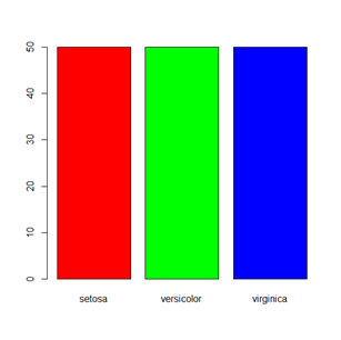
For category data, bar plot is a good choice.

> categories <- table(iris$Species)
> barplot(categories, col=c('red', 'green', 'blue'))
>


Two variable Plot

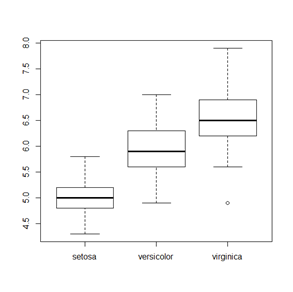
Box plot can be used to visualize the distribution of a numeric value across different categories.

> boxplot(Sepal.Length~Species, data=iris)
>
When there are multiple numeric input variables, it is useful to get an idea of their correlation to identify if there are any redundancy in our input.  Certain model is sensitive to such redundancy and won't give accurate prediction if their input has high redundancy.  This problem is known as the multicollinearity problem.

To get an idea of the correlation, we can use a scatter plot matrix for any two pairs of input variables.  We can also use a correlation matrix for the same purpose.

> # Scatter plot for all pairs
> pairs(iris[,c(1,2,3,4)])
> # Compute the correlation matrix
> cor(iris[,c(1,2,3,4)])
             Sepal.Length Sepal.Width Petal.Length Petal.Width
Sepal.Length    1.0000000  -0.1170695    0.8716902   0.8179410
Sepal.Width    -0.1170695   1.0000000   -0.4284401  -0.3661259
Petal.Length    0.8716902  -0.4284401    1.0000000   0.9628654
Petal.Width     0.8179410  -0.3661259    0.9628654   1.0000000
> 

From the observation, we can see Petal Length is highly correlated to Petal Width, and also there are some correlation between Sepal Length and Petal Width as well.

We can further drill down into analyzing the relationship between two numeric value by fitting a regression line or a regression curve (by performing local neighbor linear regression).

> # First plot the 2 variables
> plot(Petal.Width~Sepal.Length, data=iris)
> # Learn the regression model
> model <- lm(Petal.Width~Sepal.Length, data=iris)
> # Plot the regression line
> abline(model)
> # Now learn the local linear model
> model2 <- lowess(iris$Petal.Width~iris$Sepal.Length)
> lines(model2, col="red")
>


OLAP processing

If the data is in multi-dimensional form (has multiple categorical attributes), OLAP type manipulation can give a very good summary.

In this section, lets use a different data source CO2, which provides the carbon dioxide uptake in grass plants.

> head(CO2)
  Plant   Type  Treatment conc uptake
1   Qn1 Quebec nonchilled   95   16.0
2   Qn1 Quebec nonchilled  175   30.4
3   Qn1 Quebec nonchilled  250   34.8
4   Qn1 Quebec nonchilled  350   37.2
5   Qn1 Quebec nonchilled  500   35.3
6   Qn1 Quebec nonchilled  675   39.2
>

Lets look at the count summarized in different dimensions

> cube <- xtabs(~Plant+Type+Treatment, data=CO2)
> cube
, , Treatment = nonchilled

     Type
Plant Quebec Mississippi
  Qn1      7           0
  Qn2      7           0
  Qn3      7           0
  Qc1      0           0
  Qc3      0           0
  Qc2      0           0
  Mn3      0           7
  Mn2      0           7
  Mn1      0           7
  Mc2      0           0
  Mc3      0           0
  Mc1      0           0

, , Treatment = chilled

     Type
Plant Quebec Mississippi
  Qn1      0           0
  Qn2      0           0
  Qn3      0           0
  Qc1      7           0
  Qc3      7           0
  Qc2      7           0
  Mn3      0           0
  Mn2      0           0
  Mn1      0           0
  Mc2      0           7
  Mc3      0           7
  Mc1      0           7

> apply(cube, c("Plant"), sum)
Qn1 Qn2 Qn3 Qc1 Qc3 Qc2 Mn3 Mn2 Mn1 Mc2 Mc3 Mc1 
  7   7   7   7   7   7   7   7   7   7   7   7 
> apply(cube, c("Type"), sum)
     Quebec Mississippi 
         42          42 
> apply(cube, c("Plant", "Type"), mean)
     Type
Plant Quebec Mississippi
  Qn1    3.5         0.0
  Qn2    3.5         0.0
  Qn3    3.5         0.0
  Qc1    3.5         0.0
  Qc3    3.5         0.0
  Qc2    3.5         0.0
  Mn3    0.0         3.5
  Mn2    0.0         3.5
  Mn1    0.0         3.5
  Mc2    0.0         3.5
  Mc3    0.0         3.5
  Mc1    0.0         3.5
>

Prepare training data

At this step, the purpose is to transform the raw data in a form that can fit into the machine learning model.  Some common steps including ...
  • Data sampling
  • Data validation and handle missing data
  • Normalize numeric value into a uniform range
  • Compute aggregated value (a special case is to compute frequency counts)
  • Expand categorical field to binary fields
  • Discretize numeric value into categories
  • Create derived fields from existing fields
  • Reduce dimensionality
  • Power and Log transformation
Data preparation is the bulk of effort for most predictive analytic tasks and usually consumes 60 to 80% of the time.  This is an important area that deserve a dedicated post.  I'll cover data preparation in my next blog post.

Train a model

At this step, we pick a machine learning model based on the characteristics of the input and output features.  Then we feed the training data into the learning algorithm which produce a set of parameters to explain the occurrence of training data.

There are many machine learning models that we can choose from, some common ones including …
Each of the above models has its own characteristics and fit better in certain types of problems.  I'll cover each of them more detail in future posts.

Validate the model

After we train the model, how do we validate the model do a good job in prediction.  Typically, we withhold a subset of training data for testing purpose.  Through the testing, we quantitatively measure the performance of our model prediction ability.  I'll cover this topic in more detail in future post.

Deploy the model

When we are satisfied with the model, we'll deploy the model in production environment and use that to predict the real-life events.  We should also closely monitor if the real-life accuracy aligns with our testing result.

Usually, the quality of the model prediction degrades over time due to the stationary assumption (the data pattern in future is similar to the data pattern at training time) not longer holds as time passes.  On the other hand, we may acquire additional input signal that can improve the prediction accuracy.  Therefore, model should have an expiration time and need to be re-train after that.

Hopefully, this post gave a high level overview on the predictive analytics process.  I'll drill down to each items in more detail in my future posts.

Friday, April 27, 2012

Basic graph analytics using igraph

Social Network Site such as Facebook, Twitter becomes are integral part of people's life in. People interact with each other in different form of activities and a lot of information has been captured in the social network.  Mining such a network can reveal some very useful information that can help an organization to gain competitive advantages.

I recently come across a powerful tools called igraph that provides some very powerful graph mining capabilities.  Following are some interesting things that I have found.

Create a Graph

Graph is composed of Nodes and Edges, both of them can be attached with a set of properties (name/value pairs). Furthermore, edges can be directed or undirected and weights can be attached to it.
> library(igraph)
> # Create a directed graph
> g <- graph(c(0,1, 0,2, 1,3, 0,3), directed=T)
> g
Vertices: 4
Edges: 4
Directed: TRUE
Edges:

[0] 0 -> 1
[1] 0 -> 2
[2] 1 -> 3
[3] 0 -> 3
> # Create a directed graph using adjacency matrix
> m <- matrix(runif(4*4), nrow=4)
> m
[,1]      [,2]      [,3]      [,4]
[1,] 0.4086389 0.2160924 0.1557989 0.2896239
[2,] 0.4669456 0.1071071 0.1290673 0.3715809
[3,] 0.2031678 0.3911691 0.5906273 0.7417764
[4,] 0.8808119 0.7687493 0.9734323 0.4487252
> g <- graph.adjacency(m > 0.5)
> g
Vertices: 4
Edges: 5
Directed: TRUE
Edges:

[0] 2 -> 2
[1] 2 -> 3
[2] 3 -> 0
[3] 3 -> 1
[4] 3 -> 2
> plot(g, layout=layout.fruchterman.reingold)
>
iGraph also provide various convenient ways to create patterned graphs
> #Create a full graph
> g1 <- graph.full(4)
> g1
Vertices: 4
Edges: 6
Directed: FALSE
Edges:

[0] 0 -- 1
[1] 0 -- 2
[2] 0 -- 3
[3] 1 -- 2
[4] 1 -- 3
[5] 2 -- 3
> #Create a ring graph
> g2 <- graph.ring(3)
> g2
Vertices: 3
Edges: 3
Directed: FALSE
Edges:

[0] 0 -- 1
[1] 1 -- 2
[2] 0 -- 2
> #Combine 2 graphs
> g <- g1 %du% g2
> g
Vertices: 7
Edges: 9
Directed: FALSE
Edges:

[0] 0 -- 1
[1] 0 -- 2
[2] 0 -- 3
[3] 1 -- 2
[4] 1 -- 3
[5] 2 -- 3
[6] 4 -- 5
[7] 5 -- 6
[8] 4 -- 6
> graph.difference(g, graph(c(0,1,0,2), directed=F))
Vertices: 7
Edges: 7
Directed: FALSE
Edges:

[0] 0 -- 3
[1] 1 -- 3
[2] 1 -- 2
[3] 2 -- 3
[4] 4 -- 6
[5] 4 -- 5
[6] 5 -- 6
> # Create a lattice
> g1 = graph.lattice(c(3,4,2))
> # Create a tree
> g2 = graph.tree(12, children=2)
> plot(g1, layout=layout.fruchterman.reingold)
> plot(g2, layout=layout.reingold.tilford)
iGraph also provides 2 graph generation mechanism. "Random graph" is to generate an edge randomly between any two nodes. "Preferential attachment" is to assign a higher probably to create an edge to an existing node which has a high in-degree already (the rich gets richer model).
# Generate random graph, fixed probability
> g <- erdos.renyi.game(20, 0.3)
> plot(g, layout=layout.fruchterman.reingold,
  vertex.label=NA, vertex.size=5)

# Generate random graph, fixed number of arcs
> g <- erdos.renyi.game(20, 15, type='gnm')

# Generate preferential attachment graph
> g <- barabasi.game(60, power=1, zero.appeal=1.3)

Basic Graph Algorithms

This section will cover how to use iGraph to perform some very basic graph algorithm.

Minimum Spanning Tree algorithm is to find a Tree that connect all the nodes within a connected graph while the sum of edges weight is minimum.

# Create the graph and assign random edge weights
> g <- erdos.renyi.game(12, 0.35)
> E(g)$weight <- round(runif(length(E(g))),2) * 50
> plot(g, layout=layout.fruchterman.reingold, 
          edge.label=E(g)$weight)
# Compute the minimum spanning tree
> mst <- minimum.spanning.tree(g)
> plot(mst, layout=layout.reingold.tilford, 
          edge.label=E(mst)$weight)


Connected Component algorithms is to find the island of nodes that are interconnected with each other, in other words, one can traverse from one node to another one via a path.  Notice that connectivity is symmetric in undirected graph, it is not the necessary the case for directed graph (ie: it is possible that nodeA can reach nodeB, then nodeB cannot reach nodeA).  Therefore in directed graph, there is a concept of "strong" connectivity which means both nodes are considered connected only when it is reachable in both direction.  A "weak" connectivity means nodes are connected

> g <- graph(c(0, 1, 1, 2, 2, 0, 1, 3, 3, 4, 
               4, 5, 5, 3, 4, 6, 6, 7, 7, 8, 
               8, 6, 9, 10, 10, 11, 11, 9))
# Nodes reachable from node4
> subcomponent(g, 4, mode="out")
[1] 4 5 6 3 7 8
# Nodes who can reach node4
> subcomponent(g, 4, mode="in")
[1] 4 3 1 5 0 2

> clusters(g, mode="weak")
$membership
 [1] 0 0 0 0 0 0 0 0 0 1 1 1
$csize
[1] 9 3
$no
[1] 2

> myc <- clusters(g, mode="strong")
> myc
$membership
 [1] 1 1 1 2 2 2 3 3 3 0 0 0
$csize
[1] 3 3 3 3
$no
[1] 4

> mycolor <- c('green', 'yellow', 'red', 'skyblue')
> V(g)$color <- mycolor[myc$membership + 1]
> plot(g, layout=layout.fruchterman.reingold)


Shortest Path is almost the most commonly used algorithm in many scenarios, it aims to find the shortest path from nodeA to nodeB.  In iGraph, it use "breath-first search" if the graph is unweighted (ie: weight is 1) and use Dijkstra's algo if the weights are positive, otherwise it will use Bellman-Ford's algorithm for negatively weighted edges.

> g <- erdos.renyi.game(12, 0.25)
> plot(g, layout=layout.fruchterman.reingold)
> pa <- get.shortest.paths(g, 5, 9)[[1]]
> pa
[1] 5 0 4 9
> V(g)[pa]$color <- 'green'
> E(g)$color <- 'grey'
> E(g, path=pa)$color <- 'red'
> E(g, path=pa)$width <- 3
> plot(g, layout=layout.fruchterman.reingold)


Graph Statistics

There are many statistics that we can look to get a general ideas of the shape of the graph.  At the highest level, we can look at summarized statistics of the graph. This includes ...
  • Size of the graph (number of nodes and edges)
  • Density of the graph measure weither the graph dense (|E| proportional to |V|^2) or sparse (|E| proportional to |V|) ?
  • Is the graph very connected (large portion of nodes can reach each other), or is it disconnected (many islands) ?
  • Diameter of the graph measure the longest distance between any two nodes
  • Reciprocity measures in a directed graph, how symmetric the relationships are
  • Distribution of in/out "degrees"
> # Create a random graph
> g <- erdos.renyi.game(200, 0.01)
> plot(g, layout=layout.fruchterman.reingold, 
       vertex.label=NA, vertex.size=3)
> # No of nodes
> length(V(g))
[1] 200
> # No of edges
> length(E(g))
[1] 197
> # Density (No of edges / possible edges)
> graph.density(g)
[1] 0.009899497
> # Number of islands
> clusters(g)$no
[1] 34
> # Global cluster coefficient:
> #(close triplets/all triplets)
> transitivity(g, type="global")
[1] 0.015
> # Edge connectivity, 0 since graph is disconnected
> edge.connectivity(g)
[1] 0
> # Same as graph adhesion
> graph.adhesion(g)
[1] 0
> # Diameter of the graph
> diameter(g)
[1] 18
> # Reciprocity of the graph
> reciprocity(g)
[1] 1
> # Diameter of the graph
> diameter(g)
[1] 18
> # Reciprocity of the graph
> reciprocity(g)
[1] 1
> degree.distribution(g)
[1] 0.135 0.280 0.315 0.110 0.095 0.050 0.005 0.010
> plot(degree.distribution(g), xlab="node degree")
> lines(degree.distribution(g))


Drill down a level, we can also look at statistics of each pair of nodes, such as ...
  • Connectivity between two nodes measure the distinct paths with no shared edges between two nodes. (ie: how much edges need to be removed to disconnect them)
  • Shortest path between two nodes
  • Trust between two nodes (a function of number of distinct path and distance of each path)
> # Create a random graph
> g <- erdos.renyi.game(9, 0.5)
> plot(g, layout=layout.fruchterman.reingold)
> # Compute the shortest path matrix
> shortest.paths(g)
      [,1] [,2] [,3] [,4] [,5] [,6] [,7] [,8] [,9]
 [1,]    0    1    3    1    2    2    1    3    2
 [2,]    1    0    2    2    3    2    2    2    1
 [3,]    3    2    0    2    1    2    2    2    1
 [4,]    1    2    2    0    3    1    2    2    1
 [5,]    2    3    1    3    0    3    1    3    2
 [6,]    2    2    2    1    3    0    2    1    1
 [7,]    1    2    2    2    1    2    0    2    1
 [8,]    3    2    2    2    3    1    2    0    1
 [9,]    2    1    1    1    2    1    1    1    0
> # Compute the connectivity matrix
> M <- matrix(rep(0, 81), nrow=9)
> M
      [,1] [,2] [,3] [,4] [,5] [,6] [,7] [,8] [,9]
 [1,]    0    0    0    0    0    0    0    0    0
 [2,]    0    0    0    0    0    0    0    0    0
 [3,]    0    0    0    0    0    0    0    0    0
 [4,]    0    0    0    0    0    0    0    0    0
 [5,]    0    0    0    0    0    0    0    0    0
 [6,]    0    0    0    0    0    0    0    0    0
 [7,]    0    0    0    0    0    0    0    0    0
 [8,]    0    0    0    0    0    0    0    0    0
 [9,]    0    0    0    0    0    0    0    0    0
> for (i in 0:8) {
+   for (j in 0:8) {
+     if (i == j) {
+       M[i+1, j+1] <- -1
+     } else {
+       M[i+1, j+1] <- edge.connectivity(g, i, j)
+     }
+   }
+ }
> M
      [,1] [,2] [,3] [,4] [,5] [,6] [,7] [,8] [,9]
 [1,]   -1    2    2    3    2    3    3    2    3
 [2,]    2   -1    2    2    2    2    2    2    2
 [3,]    2    2   -1    2    2    2    2    2    2
 [4,]    3    2    2   -1    2    3    3    2    3
 [5,]    2    2    2    2   -1    2    2    2    2
 [6,]    3    2    2    3    2   -1    3    2    3
 [7,]    3    2    2    3    2    3   -1    2    3
 [8,]    2    2    2    2    2    2    2   -1    2
 [9,]    3    2    2    3    2    3    3    2   -1
> 

Centrality Measures

At the fine grain level, we can look at statistics of individual nodes.  Centrality score measure the social importance of a node in terms of how "central" it is based on a number of measures ...
  • Degree centrality gives a higher score to a node that has a high in/out-degree
  • Closeness centrality gives a higher score to a node that has short path distance to every other nodes
  • Betweenness centrality gives a higher score to a node that sits on many shortest path of other node pairs
  • Eigenvector centrality gives a higher score to a node if it connects to many high score nodes
  • Local cluster coefficient measures how my neighbors are inter-connected with each other, which means the node becomes less important.
> # Degree
> degree(g)
[1] 2 2 2 2 2 3 3 2 6
> # Closeness (inverse of average dist)
> closeness(g)
[1] 0.4444444 0.5333333 0.5333333 0.5000000
[5] 0.4444444 0.5333333 0.6153846 0.5000000
[9] 0.8000000
> # Betweenness
> betweenness(g)
[1]  0.8333333  2.3333333  2.3333333
[4]  0.0000000  0.8333333  0.5000000
[7]  6.3333333  0.0000000 18.8333333
> # Local cluster coefficient
> transitivity(g, type="local")
[1] 0.0000000 0.0000000 0.0000000 1.0000000
[5] 0.0000000 0.6666667 0.0000000 1.0000000
[9] 0.1333333
> # Eigenvector centrality
> evcent(g)$vector
[1] 0.3019857 0.4197153 0.4197153 0.5381294
[5] 0.3019857 0.6693142 0.5170651 0.5381294
[9] 1.0000000
> # Now rank them
> order(degree(g))
[1] 1 2 3 4 5 8 6 7 9
> order(closeness(g))
[1] 1 5 4 8 2 3 6 7 9
> order(betweenness(g))
[1] 4 8 6 1 5 2 3 7 9
> order(evcent(g)$vector)
[1] 1 5 2 3 7 4 8 6 9

From his studies, Drew Conway has found that people with low Eigenvector centrality but high Betweenness centrality are important gate keepers, while people with high Eigenvector centrality but low Betweenness centrality has direct contact to important persons.  So lets plot Eigenvector centrality against Betweenness centrality.
> # Create a graph
> g1 <- barabasi.game(100, directed=F)
> g2 <- barabasi.game(100, directed=F)
> g <- g1 %u% g2
> lay <- layout.fruchterman.reingold(g)
> # Plot the eigevector and betweenness centrality
> plot(evcent(g)$vector, betweenness(g))
> text(evcent(g)$vector, betweenness(g), 0:100, 
       cex=0.6, pos=4)
> V(g)[12]$color <- 'red'
> V(g)[8]$color <- 'green'
> plot(g, layout=lay, vertex.size=8, 
       vertex.label.cex=0.6)


With this basic of graph mining, in future posts I will cover some specific examples of social network analysis.

Sunday, April 8, 2012

Machine Learning in R: Clustering

Clustering is a very common technique in unsupervised machine learning to discover groups of data that are "close-by" to each other. It is broadly used in customer segmentation and outlier detection.

It is based on some notion of "distance" (the inverse of similarity) between data points and use that to identify data points that are close-by to each other. In the following, we discuss some very basic algorithms to come up with clusters, and use R as examples.

K-Means
This is the most basic algorithm
  1. Pick an initial set of K centroids (this can be random or any other means)
  2. For each data point, assign it to the member of the closest centroid according to the given distance function
  3. Adjust the centroid position as the mean of all its assigned member data points. Go back to (2) until the membership isn't change and centroid position is stable.
  4. Output the centroids.
Notice that in K-Means, we not only require the distance function to be defined but also requiring the mean function to be specified as well. Of course, we also need K (the number of centroids) to be specified.

K-Means is highly scalable with O(n * k * r) where r is the number of rounds, which is a constant depends on the initial pick of centroids. Also notice that the result of each round is undeterministic. The usual practices is to run multiple rounds of K-Means and pick the result of the best round. The best round is one who minimize the average distance of each point to its assigned centroid.

Here is an example of doing K-Means in R
> km <- kmeans(iris[,1:4], 3)
> plot(iris[,1], iris[,2], col=km$cluster)
> points(km$centers[,c(1,2)], col=1:3, pch=8, cex=2)
> table(km$cluster, iris$Species)

setosa versicolor virginica
1      0         48        14
2     50          0         0
3      0          2        36
with the following visual output.

Hierarchical Clustering
In this approach, it compares all pairs of data points and merge the one with the closest distance.
  1. Compute distance between every pairs of point/cluster. Compute distance between pointA to pointB is just the distance function. Compute distance between pointA to clusterB may involve many choices (such as the min/max/avg distance between the pointA and points in the clusterB). Compute distance between clusterA to clusterB may first compute distance of all points pairs (one from clusterA and the other from clusterB) and then pick either min/max/avg of these pairs.
  2. Combine the two closest point/cluster into a cluster. Go back to (1) until only one big cluster remains.
In hierarchical clustering, the complexity is O(n^2), the output will be a Tree of merge steps. It doesn't require us to specify K or a mean function. Since its high complexity, hierarchical clustering is typically used when the number of points are not too high.

Here is an example of doing hierarchical clustering in R
> sampleiris <- iris[sample(1:150, 40),]
> distance <- dist(sampleiris[,-5], method="euclidean")
> cluster <- hclust(distance, method="average")
> plot(cluster, hang=-1, label=sampleiris$Species)
with the following visual output

Fuzzy C-Means
Unlike K-Means where each data point belongs to only one cluster, in fuzzy cmeans, each data point has a fraction of membership to each cluster. The goal is to figure out the membership fraction that minimize the expected distance to each centroid.

The algorithm is very similar to K-Means, except that a matrix (row is each data point, column is each centroid, and each cell is the degree of membership) is used.
  1. Initialize the membership matrix U
  2. Repeat step (3), (4) until converge
  3. Compute location of each centroid based on the weighted fraction of its member data point's location.
  4. Update each cell as follows
Notice that the parameter m is the degree of fuzziness. The output is the matrix with each data point assigned a degree of membership to each centroids.
Here is an example of doing Fuzzy c-means in R
> library(e1071)
> result <- cmeans(iris[,-5], 3, 100, m=2, method="cmeans")
> plot(iris[,1], iris[,2], col=result$cluster)
> points(result$centers[,c(1,2)], col=1:3, pch=8, cex=2)
> result$membership[1:3,]
         1           2         3
[1,] 0.001072018 0.002304389 0.9966236
[2,] 0.007498458 0.016651044 0.9758505
[3,] 0.006414909 0.013760502 0.9798246
> table(iris$Species, result$cluster)
        1  2  3
setosa      0  0 50
versicolor  3 47  0
virginica  37 13  0
with the following visual output (very similar to K-Means)

Multi-Gaussian with Expectation-Maximization
Generally in machine learning, we will to learn a set of parameters that maximize the likelihood of observing our training data. However, what if there are some hidden variable in our data that we haven't observed. Expectation Maximization is a very common technique to use the parameter to estimate the probability distribution of those hidden variable, compute the expected likelihood and then figure out the parameters that will maximize this expected likelihood. It can be explained as follows ...

Now, we assume the underlying data distribution is based on K centroids, each a multi-variate Gaussian distribution. To map Expectation / Maximization into this, we have the following.

The order of complexity is similar to K-Means with a larger constant. It also requires K to be specified. Unlike K-Means whose cluster is always in circular shape. Multi-Gaussian can discover cluster with elliptical shape with different orientation and hence it is more general than K-Means.

Here is an example of doing multi-Gaussian with EM in R
> library(mclust)
> mc <- Mclust(iris[,1:4], 3)
> plot(mc, data=iris[,1:4], what=c('classification'),
       dimens=c(3,4))
> table(iris$Species, mc$classification)

 1  2  3
setosa     50  0  0
versicolor  0 45  5
virginica   0  0 50
with the following visual output

Density-based Cluster
In density based cluster, a cluster is extend along the density distribution. Two parameters is important: "eps" defines the radius of neighborhood of each point, and "minpts" is the number of neighbors within my "eps" radius. The basic algorithm called DBscan proceeds as follows
  1. First scan: For each point, compute the distance with all other points. Increment a neighbor count if it is smaller than "eps".
  2. Second scan: For each point, mark it as a core point if its neighbor count is greater than "minpts"
  3. Third scan: For each core point, if it is not already assigned a cluster, create a new cluster and assign that to this core point as well as all of its neighbors within "eps" radius.
Unlike other cluster, density based cluster can have some outliers (data points that doesn't belong to any clusters). On the other hand, it can detect cluster of arbitrary shapes (doesn't have to be circular at all)

Here is an example of doing DBscan in R
> library(fpc)
# eps is radius of neighborhood, MinPts is no of neighbors
# within eps
> cluster <- dbscan(sampleiris[,-5], eps=0.6, MinPts=4)
> plot(cluster, sampleiris)
> plot(cluster, sampleiris[,c(1,4)])
# Notice points in cluster 0 are unassigned outliers
> table(cluster$cluster, sampleiris$Species)

setosa versicolor virginica
0      1          2         6
1      0         13         0
2     12          0         0
3      0          0         6
with the following visual output ... (notice the black points are outliers, triangles are core points and circles are boundary points)

Although this has covered a couple ways of finding cluster, it is not an exhaustive list. Also here I tried to illustrate the basic idea and use R as an example. For really large data set, we may need to run the clustering algorithm in parallel. Here is my earlier blog about how to do K-Means using Map/Reduce as well as Canopy clustering as well.

Monday, April 2, 2012

MongoDb Architecture

NOSQL has become a very heated topic for large web-scale deployment where scalability and semi-structured data driven the DB requirement towards NOSQL. There has been many NOSQL products evolving in over last couple years. In my past blogs, I have been covering the underlying distributed system theory of NOSQL, as well as some specific products such as CouchDB and Cassandra/HBase.

Last Friday I was very lucky to meet with Jared Rosoff from 10gen in a technical conference and have a discussion about the technical architecture of MongoDb. I found the information is very useful and want to share with more people.

One thing I am very impressed by MongoDb is that it is extremely easy to use and the underlying architecture is also very easy to understand.

Here are some simple admin steps to start/stop MongoDb server
# Install MongoDB
mkdir /data/lib

# Start Mongod server
.../bin/mongod # data stored in /data/db

# Start the command shell
.../bin/mongo
> show dbs
> show collections

# Remove collection
> db.person.drop()

# Stop the Mongod server from shell
> use admin
> db.shutdownServer()

Major difference from RDBMS
MongoDb differs from RDBMS in the following way
  • Unlike an RDBMS record which is "flat" (a fixed number of simple data type), the basic unit of MongoDb is "document" which is "nested" and can contain multi-value fields (arrays, hash).
  • Unlike RDBMS where all records stored in a table must be confined to the table schema, documents of any structure can be stored in the same collection.
  • There is no "join" operation in the query. Overall, data is encouraged to be organized in a more denormalized manner and the more burden of ensuring data consistency is pushed to the application developers
  • There is no concept of "transaction" in MongoDb. "Atomicity" is guaranteed only at the document level (no partial update of a document will occurred).
  • There is no concept of "isolation", any data read by one client may have its value modified by another concurrent client.
By removing some of those features that a classical RDBMS will provide, MongoDb can be more light-weight and be more scalable in processing big data.
Query processingMongoDb belongs to the type of document-oriented DB. In this model, data is organized as JSON document, and store into a collection. Collection can be thought for equivalent to Table and Document is equivalent to records in RDBMS world.

Here are some basic example.
# create a doc and save into a collection
> p = {firstname:"Dave", lastname:"Ho"}
> db.person.save(p)
> db.person.insert({firstname:"Ricky", lastname:"Ho"})

# Show all docs within a collection
> db.person.find()

# Iterate result using cursor
> var c = db.person.find()
> p1 = c.next()
> p2 = c.next()

To specify the search criteria, an example document containing the fields that needs to match against need to be provided.
> p3 = db.person.findone({lastname:"Ho"})
Notice that in the query, the value portion need to be determined before the query is made (in other words, it cannot be based on other attributes of the document). For example, lets say if we have a collection of "Person", it is not possible to express a query that return person whose weight is larger than 10 times of their height.
# Return a subset of fields (ie: projection)
> db.person.find({lastname:"Ho"}, {firstname:true})

# Delete some records
> db.person.remove({firstname:"Ricky"})
To speed up the query, index can be used. In MongoDb, index is stored as a BTree structure (so range query is automatically supported). Since the document itself is a tree, the index can be specified as a path and drill into deep nesting level inside the document.
# To build an index for a collection
> db.person.ensureIndex({firstname:1})

# To show all existing indexes
> db.person.getIndexes()

# To remove an index
> db.person.dropIndex({firstname:1})

# Index can be build on a path of the doc.
> db.person.ensureIndex({"address.city":1})

# A composite key can be used to build index
> db.person.ensureIndex({lastname:1, firstname:1})
Index can also be build on an multi-valued attribute such as an array. In this case, each element in the array will have a separate node in the BTree.

Building an index can be done in both offline foreground mode or online background mode. Foreground mode will proceed much faster but the DB cannot be access during the build index period. If the system is running in a replica set (describe below), it is recommended to rotate each member DB offline and build the index in foreground.

When there are multiple selection criteria in a query, MongoDb attempts to use one single best index to select a candidate set and then sequentially iterate through them to evaluate other criteria.

When there are multiple indexes available for a collection. When handling a query the first time, MongoDb will create multiple execution plans (one for each available index) and let them take turns (within certain number of ticks) to execute until the fastest plan finishes. The result of the fastest executor will be returned and the system remembers the corresponding index used by the fastest executor. Subsequent query will use the remembered index until certain number of updates has happened in the collection, then the system repeats the process to figure out what is the best index at that time.

Since only one index will be used, it is important to look at the search or sorting criteria of the query and build additional composite index to match the query better. Maintaining an index is not without cost as index need to be updated when docs are created, deleted and updated, which incurs overhead to the update operations. To maintain an optimal balance, we need to periodically measure the effectiveness of having an index (e.g. the read/write ratio) and delete less efficient indexes.

Storage Model
Written in C++, MongoDB uses a memory map file that directly map an on-disk data file to in-memory byte array where data access logic is implemented using pointer arithmetic. Each document collection is stored in one namespace file (which contains metadata information) as well as multiple extent data files (with an exponentially/doubling increasing size).
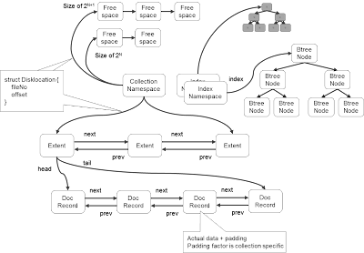

The data structure uses doubly-linked-list extensively. Each collection of data is organized in a linked list of extents each of which represents a contiguous disk space. Each extent points to a head/tail of another linked list of docs. Each doc contains a linked list to other documents as well as the actual data encoded in BSON format.

Data modification happens in place. In case the modification increases the size of record beyond its originally allocated space, the whole record will be moved to a bigger region with some extra padding bytes. The padding bytes is used as an growth buffer so that future expansion doesn't necessary require moving the data again. The amount of padding is dynamically adjusted per collection based on its modification statistics. On the other hand, the space occupied by the original doc will be free up. This is kept tracked by a list of free list of different size.

As we can imagine holes will be created over time as objects are created, deleted or modified, this fragmentation will hurt performance as less data is being read/write per disk I/O. Therefore, we need to run the "compact" command periodically, which copy the data to a contiguous space. This "compact" operation however is an exclusive operation and has to be done offline. Typically this is done in a replica setting by rotating each member offline one at a time to perform the compaction.

Index are implemented as BTree. Each BTree node contains a number of keys (within this node), as well as pointers to left children BTree nodes of each key.

Data update and Transaction
To update an existing doc, we can do the following
var p1 = db.person.findone({lastname:"Ho"})
p1["address"] = "San Jose"
db.person.save(p1)

# Do the same in one command
db.person.update({lastname:"Ho"},
              {$set:{address:"San Jose"}},
              false,
              true)
Write by default doesn't wait. There are various wait options that the client can specified what conditions to wait before the call returns (this can also achievable by a followup "getlasterror" call), such as where the changes is persisted on disk, or changes has been propagated to sufficient members in the replica set. MongoDb also provides a sophisticated way to assign tags to members of replica set to reflect their physical topology so that customized write policy for each collection can be made based on their reliability requirement.

In RDBMS, "Serializability" is a very fundamental concept about the net effect of concurrently executing work units is equivalent to as if these work units are arrange in some order of sequential execution (one at a time). Therefore, each client can treat as if the DB is exclusively available. The underlying implementation of DB server many use LOCKs or Multi-version to provide the isolation. However, this concept is not available in MongoDb (and many other NOSQL as well)

In MongoDb, every data you read should be treated as a snapshot of the past, which means by the time you look at it, it may have been changed in the DB. Therefore, if you are making a modification based on some previously read data, by the time you send the modification request, the condition where your modification is based on may have changed. If this is not acceptable for your application's consistency requirement, you may need to re-validate the condition at the time you request the modification (ie: a "conditional_modify" should be made).

Under this scheme, a "condition" is attached along with the modification request so that the DB server can validate the condition before applying the modification. (of course, the condition checking and modification must be atomic so no update can happen in between). In MongoDb, this can be achieved by the "findAndModify" call.
var account = db.bank.findone({id:1234})
var old_bal = account['balance']
var new_bal = old_bal + fund

# Pre-condition is specified in search criteria
db.bank.findAndModify({id:1234, balance:old_bal},
                   {$set: {balance: new_bal}})

# Check if the prev command successfully
var success =
   db.runCommand({getlasterror:1,j:true})

if (!success) {
 #retry_from_beginning
}
The concept of "transaction" is also missing in MongoDb. While MongoDb guarantee each document will be atomically modified (so no partial update will happen within a doc), but if the update modifies multiple documents, then there are no guarantee on the atomicity across documents.

Therefore, it is the application developers responsibility to implement the multi-update atomicity across multiple documents. We describe a common design pattern to achieve that. This technique is not specific to MongoDb and applicable to other NOSQL store, which can at least guarantee atomicity at the single record level.

The basic idea is to first create a separate document (called transaction) that links together all the documents that you want to modify. And then create a reverse link from each document (to be modified) back to the transaction. By carefully design the sequence of update in the documents and the transaction, we can achieve the atomicity of modifying multiple documents.
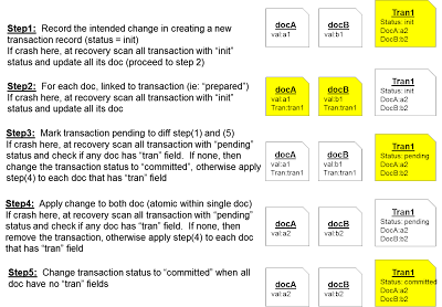

MongoDb's web site has also described a similar technique here (based on the same concept but the implementation is slightly different).

Replication Model
High availability is achieved in MongoDb via Replica Set, which provides data redundancy across multiple physical servers, including a single primary DB as well as multiple secondary DBs. For data consistency, all modifications (insert / update / deletes) request go to the primary DB where modification is made and asynchronously replicated to the other secondary DBs.
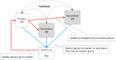

Within the replica set, members are interconnected with each other to exchange heartbeat message. A crashed server with missing heartbeat will be detected by other members and removed from the replica set membership. After the dead secondary recovers in future, it can rejoin the cluster by connecting to the primary to catchup the latest update since its last crashed. If the crashes happens in a lengthy period of time where the change log from the primary doesn't cover the whole crash period, then the recovered secondary need to reload the whole data from the primary (as if it was a brand new server).

In case of the primary DB crashes, a leader election protocol will be run among the remaining members to nominate the new primary, based on many factors such as the node priority, node uptime ... etc. After getting majority vote, the new primary server will take place. Notice that due to async replication, the newly elected primary DB doesn't necessary having all the latest updated from the crashed DB.

Client lib provides the API for the App to access the MongoDB server. At startup, the client lib will connect to some member (based on a seed list) of the Replica set and issue a "isMaster" command to gather the current picture of the set (who is the primary and secondaries). After that, the client lib connect to the single primary (where it will send all DB modification request) and some number of secondaries (where it will send read-only queries). The client library will periodically re-run the "isMaster" command to detect if any new members has joined the set. When an existing member in the set is crashed, connections to all existing clients will be dropped and forces a resynchronization of the latest picture.

There is also a special secondary DB called slave delay, which guarantee the data is propagated with a certain time lag with the master. This is used mainly to recover data after accidental deletion of data.

For data modification request, the client will send the request to the primary DB, by default the request will be returned once written to the primary, an optional parameter can be specified to indicate a certain number of secondaries need to receive the modification before return so the client can ensure the majority portion of members have got the request. Of course there is a tradeoff between latency and reliability.

For query request, by default the client will contact the primary which has the latest updated data. Optionally, the client can specify its willingness to read from any secondaries, and tolerate that the returned data may be outdated. This provide an opportunity to load balance the read request across all secondaries. Notice that in this case, a subsequent read following a write may not seen the update.

For read-mostly application, reading form any secondaries can be a big performance improvement. To select the fastest secondary DB member to issue query, the client driver periodically pings the members and will favor issuing the query to the one with lowest latency. Notice that read request is issued to only one node, there is no quorum read or read from multiple nodes in MongoDb.

The main purpose of Replica set is to provide data redundancy and also load balance read-request. It doesn't provide load balancing for write-request since all modification still has to go to the single master.

Another benefit of replica set is that members can be taken offline on an rotation basis to perform expensive operation such as compaction, indexing or backup, without impacting online clients using the alive members.

Sharding Model
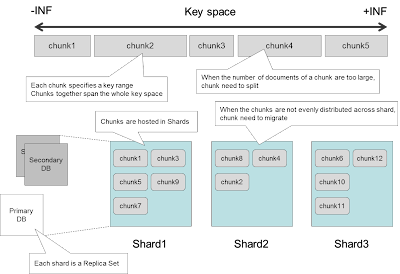
To load balance write-request, we can use MongoDb shards. In the sharding setup, a collection can be partitioned (by a partition key) into chunks (which is a key range) and have chunks distributed across multiple shards (each shard will be a replica set). MongoDb sharding effectively provide an unlimited size for data collection, which is important for any big data scenario.

To reiterate, in the sharding model, a single partition key will be specified for each collection that is stored in the sharding cluster. The key space of the partition key is divided into contiguous key range called chunk, which is hosted by corresponding shards.

# To define the partition key
db.runcommand({shardcollection: "testdb.person",
         key: {firstname:1, lastname:1}})
In the shard setting, the client lib connects to a stateless routing server "MongoS", which behaves as if the "MongoD". The routing server plays an important role in forwarding the client request to the appropriate shard server according to the request characteristics.
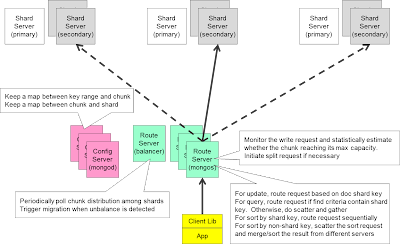

For insert/delete/update request containing the partition key, based on the chunk/shard mapping information (obtained from the config Server and cache locally), the route server will forward the request to the corresponding primary server hosting the chunk whose key range covers the partition key of the modified doc. Given a particular partition key, the primary server containing that chunk can be unambiguously determined.

In case of query request, the routing server will examine whether the partition key is part of the selection criteria and if so will only "route" the request to the corresponding shard (primary or secondary). However, if the partition key is not part of the selection criteria, then the routing server will "scatter" the request to every shard (pick one member of each shard) which will compute its local search, and the result will be gathered at the routing server and return to the client. When the query requires the result to be sorted, and if the partition key is involved in the sort order, the routing server will route the request sequentially to multiple shards as the client iterate the result. In case the sort involves other key which is not the partition key, the router server will scatter the request to all shards which will perform its local sort, and then merge the result at the routing server (basically a distributed merge-sort).

As data are inserted into chunk and get close to its full capacity, we need to split the chunk. The routing server can detect this situation statistically based on the number of requests it forward as well as the number of other routing server exist. Then the routing server will contact the primary server of the shard that contains the full chunk and request for a chunk split. The shard server will compute the mid point of the key range that can evenly distribute the data and then split the chunk and update the configuration server about its split point. Notice that so far there is no data movement as data is still residing in the same shard server.

On the other hand, there is another "balancer" process (running in one of the routing server) whose job is to make sure each shard carry approximately same number of chunks. When the unbalance condition is detected, the balancer will contact the busy shard to trigger a chunk migration process. This migration process happens online where the origination contacts the destination to initiate a data transfer, and data will start to be copied from the origination to the destination. This process may take some time (depends on the data volume) during which update can happen continuously at the origination. These changes will be tracked at the origination and when the copy finishes, delta will then transfer and applied to the destination. After multiple rounds of applying deltas, the migration enters the final round and the origination will halt and withhold all request coming from the routing server. After the last round of changes have been applied to the destination, the destination will update the configuration server about the new shard configuration and notify the origination shard (which is still withholding the request) to return a StaleConfigException to the Routing server, which will then re-read the latest configuration from the configServer and re-submit the previous requests. At some future point in time, data at the origination will be physically deleted.

It is possible that under a high frequency update condition, the changes being applied to the destination is unable to catch up with the update rate happen at the origination. When this situation is detected, the whole migration process will be aborted. The routing server may pick a different chunk to start the migration afterwards.

Map/Reduce Execution
MongoDb provide a Map/Reduce framework to perform parallel data processing. The concept is similar to Hadoop Map/Reduce, but with the following small differences ...
  • It takes input from the query result of a collection rather than HDFS directory
  • The reduce output can be append to an existing collection rather than an empty HDFS directory
Map/Reduce in Mongo works in a slightly different way as follows
  1. Client define a map function, reduce function, query that scope the input data, and an output collection that store the output result.
  2. Client send the request to the MongoS routing server
  3. MongoS forward the request to the appropriated shards (route or scatter depends on whether partition key appears in the query). Notice that MongoS will pick one member of each shard, currently always send to the primaryDB
  4. Primary DB of each shard executes the query and pipe output to the user-defined map function, which emit a bunch of key value pairs stored in memory buffer. When the memory buffer is full, a user-defined reducer function will be invoked that partially reduce the key values pairs in the memory buffer, result stored on the local collection.
  5. When step (4) completes, the reduce function will be executed on all the previous partially reduced result to merge a single reduced result on this server.
  6. When step (5) finishes, MongoS notifies the corresponding shard servers that will store the output collection. (if the output collection is non-partitioned, only a single shard will be notified, otherwise all shards will be notified).
  7. The primary db of the shard(s) storing the final collection will call for every shard to collect the partially reduced data previously done. It will only ask for the result based on its corresponding key range.
  8. The primary db run the reduce() function again on the list of partially reduced result. Then store the final reduced result locally. If the user provide a finalize function, it will be invoked as well.
Here is a simple example to build an inverted index from document to topics
db.book.insert({title:"NOSQL",
             about:["software", "db"]})

db.book.insert({title:"Java programming",
             about:["software", "program"]})

db.book.insert({title:"Mongo",
             about:["db", "technology"]})

db.book.insert({title:"Oracle",
             about:["db", "software"]})

db.book.find()

m = function() {
 for (var i in this.about) {
     emit(this.about[i], this.title)
 }
}

r = function(k, vals) {
 return({topic:k, title:vals})
}

db.book.mapReduce(m, r, {query:{},
               out:{replace:"mroutput"}})

db.mroutput.find()
Overall speaking, I found MongoDb is very powerful and easy to use. I look forward to use MongoDb with Node.js and will share my experience in future blogs.

Especially thanks to Jared Rosoff who provides me a lot of details of how MongoDb is implemented.

Tuesday, March 6, 2012

Designing robust web API

Many companies over the past years have been exposing their services via web service API. Some are doing a better job than the other. Once the API s publicly available, people will write code based on it, every change will break the client and make them unhappy. It is very important to get the first version of your API right.

In this post, I summarize some good practices that I have used successfully in my previous projects.

Use a RESTful Model
Design the web service API model on HTTP, REST and JSON format.
There has been a lot of comparison between SOAP and REST that I don't want to repeat here. The winner is surely REST. In this "resource oriented model", every resource type will be represented as a collection. On the other hand, HTTP verbs will be used to manipulate the resources.

Restful URL typically comes with the collection URI as well the individual URI. Here are some common examples for a resource type Person:
  1. List all persons. GET /persons
  2. Find a person with a particular id. GET /persons/123
  3. Get partial fields. GET /persons/123?fields=(name,age)
  4. Find a person's particular friend. GET/persons/123/friends/456
  5. Find all persons named John. GET /persons/search?q=(name,eq,John)
  6. Find all dogs whose master is John. GET /persons/search?q=(name,eqJohn)/dogs
  7. Create a person with a server assigned id. POST /persons?name=Dave&age=10
  8. Create a person with a client assigned id. PUT /persons/123?name=Dave&age=10
  9. Ask the person to perform an action. POST /persons/123/action/travel?location=Euro
  10. Remove a person. DELETE /persons/123
  11. Return a page of result. GET /persons/search?q=(name,eq,John)&offset=1&limit=25
It is a good practice to categorize the API based on whether it is cacheable and whether it is idempotent. Cacheable API is typically implemented using HTTP GET, whose response can be cached somewhere and can be reused in subsequent request. Notice that cacheable API can help reducing the workload on the server, but on the other hand, not accurately tracking the actual usage of the client. Idempotent API can be invoked multiple times with the same effect of being invoked once, which is important in unreliable network where retry is very common. POST is the only mechanism to implement non-idempotent API.
For input parameters, I tend to put everything into the URL and not using the HTTP headers, which is used for OAuth headers.
In case of any error happens, it should fail fast and communicate the error clearly to the calling user. HTTP error code should be used for this purpose; response code 200 is typically used if the request is processed successfully; response code 400 is used if the server runs into some application logic problem; response code 500 is used if the API request send by the client is wrong. A human readable error message, together with the hint to fix that, should be sent back in the HTTP body response.
For those who is interested in seeing more examples, here is an earlier blog that I wrote.
Stabilize your APIAPI is public and hence must be stable. To achieve the stability, the API should expose as minimal as possible (notice it is much easier to add stuff later but very difficult to remove anything that you have expose). Also, the API should only expose the function semantics but nothing about its implementation details, which allows the implementation to continuously evolve without breaking the client interface. There is actually a development practice that I advocate about having the architect to write API interface that confines the functional expectation of every system component. API designed in this way usually ends up with a higher level of abstraction.

A good API should focus to do one thing well, rather than multiple things of different purposes. Each API must be self-contained and not relying on any specific call sequence to work correctly. The only exception is the authentication call which must the first call to make and precede any other application API calls. As far as API security, App level key, with OAuth2.0 protocol should be used for authentication and authorization purpose.

It should also be very intuitive to use and difficult to make undetected mistakes without needing to read through the documentation. This usually requires the API to have a high degree of consistency (such as parameter ordering, naming convention etc) as well as short but clear documentation with simple usage example code.

On the development process side, we should let more people to review the API design, and perhaps run some pilot client projects before exposing it to the general public.

Version your APIEven you try to stablise your API, change will still be needed over time. This can be due to new requirements that you don't originally expected has arrived.

If you follow the minimal API design approach, the newer version is usually about adding parameters to your original API rather than removing parameters. A good practice is to support both API interface (the older version as well as the newer version) behind the same URL. (e.g. http://xyz.com/v1/path/...). On the implementation side, you only have the implementation that takes the latest version API parameters as input. In other words, you are prepared to receive request of the older version as well as the latest version. But you substitute the default value of the parameters of the newer version that is missing in the older version. And then send this request (with all the parameters filled) to the latest implementation.

Notice that by keeping the original endpoint URL unchanged, you are committed to provide backward compatibility (able to handle an older version request).

If your later version of API have an incompatible change (e.g. having a new parameter that is mandatory). The general practice is to use a different URL endpoint for the new version (e.g. http://xyz.com/v2/path/...). You also keep the corresponding implementation (v1 and v2) behind those endpoints. Depends on your decision whether to keep supporting the older version, you may want to introduce a deprecation process. Unfortunately there is no standard way to indicate an API will be deprecated in the response. One possible way is to put a flag in the HTTP header of the response to indicate when the API will be deprecated.

Asynchronous Invocation
Most API tend to be synchronous which means the client makes a call, wait until the server finishes the processing and return the result. But if the server takes a longer time to finish its processing, then an asynchronous invocation mechanism is important.

One simple mechanism is the client request is immediately returned with a receipt, while the server queue up the request and processing it at a later time. The receipt will be used by the client later to poll the server with the processing status and claim the result once it is available.

Another mechanism is to have the client provide a callback address in its request, which gets return immediately. After the server finishes the processing at a later time, it will invoke the callback address to push the result back to the client. While this is more resource efficient than the polling mechanism above, it involves more setup on the client side, such as running the server to listen for callbacks, and make sure the server can be authenticated in its callback.

Sunday, February 19, 2012

Characteristics of Machine Learning Model

I was motivated to write this blog from a discussion on the Machine Learning Connection group

For classification and regression problem, there are different choices of Machine Learning Models each of which can be viewed as a blackbox that solve the same problem. However, each model come from a different algorithm approaches and will perform differently under different data set. The best way is to use cross-validation to determine which model perform best on test data.

Here I'll try to provide a high level summary of its underlying algorithmic approach and hopefully can give a sense of whether it will be a good fit for your particular problem.


Decision Tree based methods
The fundamental learning approach is to recursively divide the training data into buckets of homogeneous members through the most discriminative dividing criteria. The measurement of "homogeneity" is based on the output label; when it is a numeric value, the measurement will be the variance of the bucket; when it is a category, the measurement will be the entropy or gini index of the bucket. During the learning, various dividing criteria based on the input will be tried (using in a greedy manner); when the input is a category (Mon, Tue, Wed ...), it will first be turned into binary (isMon, isTue, isWed ...) and then use the true/false as a decision boundary to evaluate the homogeneity; when the input is a numeric or ordinal value, the lessThan, greaterThan at each training data input value will be used as the decision boundary. The training process stops when there is no significant gain in homogeneity by further split the Tree. The members of the bucket represented at leaf node will vote for the prediction; majority wins when the output is a category and member average when the output is a numeric.

The good part of Tree is that it is very flexible in terms of the data type of input and output variables which can be categorical, binary and numeric value. The level of decision nodes also indicate the degree of influences of different input variables. The limitation is each decision boundary at each split point is a concrete binary decision. Also the decision criteria only consider one input attributes at a time but not a combination of multiple input variables. Another weakness of Tree is that once learned it cannot be updated incrementally. When new training data arrives, you have to throw away the old tree and retrain every data from scratch.

However, Tree when mixed with Ensemble methods (e.g. Random Forest, Boosting Trees) addresses a lot of the limitations mentioned above. For example, Gradient Boosting Decision Tree consistently beat the performance of other ML models in many problems and is one of the most popular method these days.

Linear regression based methods
The basic assumption is that the output variable (a numeric value) can be expressed as a linear combination (weighted sum) of a set of input variable (which is also numeric value).
y = w1x1 + w2x2 + w3x3 ....

The whole objective of the training phase is to learn the weights w1, w2 ... by minimizing the error function lost(y, w1x1 + w2x2 + ...). Gradient descent is the classical technique of solving this problem with the general idea of adjusting w1, w2 ... along the direction of the maximum gradient of the loss function.

The input variable is required to be numeric. For binary variable, this will be represented as 0, 1. For categorical variable, each possible value will be represented as a separate binary variable (and hence 0, 1). For the output, if it is a binary variable (0, 1) then a logit function is used to transform the range of -infinity to +infinity into 0 to 1. This is called logistic regression and a different loss function (based on maximum likelihood) is used.

To avoid overfitting, regularization technique (L1 and L2) is used to penalize large value of w1, w2 ... L1 is by adding the absolute value of w1 into the loss function while L2 is by adding the square of w1 into the loss function. L1 has the property that it will penalize redundant features or irrelevant feature more (with very small weight) and is a good tool to select highly influential features.

The strength of Linear model is that it has very high performance in both scoring and learning. The Stochastic gradient descent-based learning algorithm is highly scalable and can handle incremental learning.

The weakness of linear model is linear assumption of input features, which is often false. Therefore, an important feature engineering effort is required to transform each input feature, which usually involved domain expert. Another common way is to throw different transformation functions 1/x, x^2, log(x) in the hope that one of them will have a linear relationship with the output. Linearity can be checked by observing whether the residual (y - predicted_y) is normally distributed or not (using the QQplot with the Gaussian distribution).

Neural Network
Neural Network can be considered as multiple layer of perceptron (each is a logistic regression unit with multiple binary input and one binary output). By having multiple layers, this is equivalent to : z = logit(v1.y1 + v2y2 + ...), while y1 = logit(w11x1 + w12x2 + ...)

This multi-layer model enables Neural Network to learn non-linear relationship between input x and output z. The typical learning technique is "backward error propagation" where the error is propagate from the output layer back to the input layer to adjust the weight.

Notice that Neural Network expect binary input which means we need to transform categorical input into multiple binary variable. For numeric input variable, we can transform that into binary encoded 101010 string. Categorical and numeric output can be transformed in a similar way.

Bayesian Network
It is basically a dependency graph where each node represents a binary variable and each edge (directional) represents the dependency relationship. If NodeA and NodeB has an edge to NodeC. This means the probably of C is true depends on different combinations of the boolean value of A and B. NodeC can point to NodeD and now NodeD depends on NodeA and NodeB as well.

The learning is about finding at each node the join-probability distribution of all incoming edges. This is done by counting the observed values of A, B and C and then update the joint probability distribution table at NodeC.

Once we have the probability distribution table at every node, then we can compute the probability of any hidden node (output variable) from the observed nodes (input variables) by using the Bayes rule.

The strength of Bayesian network is it is highly scalable and can learn incrementally because all we do is to count the observed variables and update the probability distribution table. Similar to Neural Network, Bayesian network expects all data to be binary, categorical variable will need to be transformed into multiple binary variable as described above. Numeric variable is generally not a good fit for Bayesian network.

Support Vector Machine
Support Vector Machine takes numeric input and binary output. It is based on finding a linear plane with maximum margin to separate two class of output. Categorical input can be turned into numeric input as before and categorical output can be modeled as multiple binary output.

With a different lost function, SVM can also do regression (called SVR). I haven't used this myself so I can't talk much.

The strength of SVM is it can handle large number of dimensions. With the kernel function, it can handle non-linear relationship as well.

Nearest Neighbor
We are not learning a model at all. The idea is to find K similar data point from the training set and use them to interpolate the output value, which is either the majority value for categorical output, or average (or weighted average) for numeric output. K is a tunable parameter which needs to be cross-validated to pick the best value.

Nearest Neighbor require the definition of a distance function which is used to find the nearest neighbor. For numeric input, the common practice is to normalize them by minus the mean and divided by the standard deviation. Euclidean distance is commonly used when the input are independent, otherwise mahalanobis distance (which account for correlation between pairs of input features) should be used instead. For binary attributes, Jaccard distance can be used.

The strength of K nearest neighbor is its simplicity as no model needs to be trained. Incremental learning is automatic when more data arrives (and old data can be deleted as well). Data, however, needs to be organized in a distance-aware tree such that finding the nearest neighbor is O(logN) rather than O(N). On the other hand, the weakness of KNN is it doesn't handle high number of dimensions well. Also, the weighting of different factors needs to be hand tuned (by cross-validation on different weighting combination) and can be a very tedious process.

Saturday, January 14, 2012

Machine Learning: Ensemble Methods

Ensemble Method is a popular approach in Machine Learning based on the idea of combining multiple models. For example, by mixing different machine learning algorithms (e.g. SVM, Logistic regression, Bayesian network), ensemble method can automatically pick the best algorithmic model that fits the data the best. On the other hand, by mixing different parameter set of the same algorithmic model (e.g. Random forest, Boosting tree), it can pick the best set of parameters of the same algorithmic model.

Bagging
Bagging is based on the idea of learning multiple models using different sets of sample data, basically by random sampling (with replacement) from the same training set. After the models are learned, we use a voting scheme to predict future data. In case of the classification problem, we use the majority class voted by all models. In case of the regression problem, we take the average value of estimated output from all models.

The model doesn't have to be equally weighted. We can use a weighted average of individual models to come up with the final model. m = w1.m1 + w2.m2 + w3.m3 + ...

To obtain the weights w1, w2 ... we can use machine learning to figure out. In the case, we first use the training data set to train individual models. After that, we use the validation data set to train the weights. Concretely, we feed each data point from the validation set to each model to come up with the final prediction. Based on how the ensembled prediction deviates from the actual outcome, we can learn the optimal set of weights.

Boosting
Boosting extend the idea of bagging by putting more emphasis on the training data that is wrongly predicted. In boosting, weight sampling is used. Initially each training data is equally weighted but as each iteration goes, the data that is wrongly classified will have its weight increased. On the other hand, the model also has its weighted according to how good this model is predicting the data in its round.
  1. Each training data carry a sample weight (initially are the same)
  2. For each iteration, take sample (with replacement) based on weights
  3. Compute the error rate e
  4. For each sample that is wrongly predicted, adjust its sample weight by e/(1-e)
  5. Weight the trained model according to its error. For example, log(e/(1-e))
  6. Stop when e is small enough
  7. Ensemble the overall model according to model weight.
Gradient Boosting Method is one of the most powerful and popular boosting methods. It is based on incrementally add a function that fits the residuals.

Found function F to fit y ~ F(x) using a gradient descent approach.

Start with some random guessing function F. Compute the loss based on the residual.
loss = L(y - F(x)) where L is some loss function

Partial differentiate loss w.r.t. function F, and compute the value at every data point. Use another machine learning model to learn another function g(x) that predicts the partial differentiation value. Then update F(x) <- F(x) + a.g(x) where a is the learning rate.

Other ways of Sampling
Instead of sampling the training data, we can also sample on the attributes (e.g. we can randomly pick a subset of the input variables) Random Forest is an example of this approach.

Sliding window
Machine Learning is based on an important assumption that the future is repeating the same pattern as the history. As we all know, as time goes by, this assumption becomes more and more invalid. In other words, we should put more weight in recent history than long term history.

Ensemble method also gives us an elegant way to decay the weight of old data. In this case, we maintain a sliding window of models (say the last 7 days). We learn a model daily and expire the oldest model we compute 7 days ago.

M = M1 + M2.a + M3.a^2 + ... + M7.a^6
M = M / (1 + a + a^2 + ... + a^6)