Structure Learning and Imitation Learning

In classical prediction use case, the predicted output is either a number (for regression) or category (for classification).  A set of training data (x, y) where x is the input and y is the labeled output is provided to train a parameterized predictive model.

• The model is characterized by a set of parameters w
• Given an input x, for the model predicts y_hat = f(x; w) for regression, or the model predicts the probability of each possible class for classification
• Define a Lost function L(y, y_hat) for regression, or L(y, P(y=a | x), P(y=b | x) ...), find the parameters w to minimize L

This problem is typically view as an optimization problem, and use gradient descent approach to solve it.

Need for Structure Learning

However, in some cases, y is not as simple as a number or a class.  For example

• For machine translation, x is a sentence in English, and y is a translated sentence in French
• For self-driving-vehicle, x is a camera image, and y is the control action on steering wheel, brake, gas pedal

In these cases, the output y can be viewed as an object.  But wait, can we break down the object as multiple numbers / categories and use the classical regression / classification approach to solve it ?  Not quite, because the lost function cannot be just formulated as the summation of loss of individual components.  For example, two French sentences using different words may still be a very good translation of the same English sentence.  So we need to generalize a bit more and introduce the concept of an object and compatibility here.

The prediction problem can be generalized as: Given input x, finding an object y such that y is the "most compatible" with x.  The compatibility is a parameterized function that we are going to learn from the training data.

• The compatibility function is defined as F(x, y; w)
• During training phase, we tune parameter w such that for every sample in training data, F(x, y; w) is the maximum.  In other words, F(x, Y=y; w) > F(x, Y=other_val; w)

Notice that the training process is different from classical ML in the following way.

• There are two optimization loop here.  a) Given parameter w, find y_opt that maximize F(x,y,w).  b) Given Lost = gap between F(x,y,w) and F(x,y_opt,w), find w that minimize the gap.
• It turns out the first optimization is solved in a problem specific way while the second optimization can be solved by classical gradient descent approach.

After we learn the compatibility function parameters, at inference phase, we will apply the first optimization to the given input x to find the most compatible y_opt such that F(x, y_opt; w) is the maximum.

Rather than trying to exactly match y_hat to y in the training data, structure learning enable us to learn a more abstract relationship (ie: compatibility) between x and y so that we can output other equally-good y even it is not the same as the y in the training data.  This more-generalized form is very powerful when we don't have a lot of training data.  The downside of structure learning is it is compute intensive, because at inference phase it needs to solve an optimization problem which is typically expensive.

Imitation Learning

In a typical setting of Reinforcement Learning, an digital agent observe the state from the environment, formulate its policy to determine an action that it believes will maximize its accumulative future reward, take the action, get the reward from the environment and transition to the next state.  Reinforcement learning is about how the agent optimize its policy along its experience when interacting with the environment.

For an overview of Reinforcement Learning and basic algorithm, you can visit my previous blog here.

Basically, reinforcement learning is based on a trial-and-error approach to learn the lesson.  This approach can be very costly because during the trial process, serious mistake can be made (imagine if we use reinforcement learning to learn self-driving car, we may crash many cars before we learn something meaningful).  In practice, people rely on simulator to mimic the environment.  However, coming up good simulator is not easy because it requires a very deep understanding of how the actual environment behaves, this is one of the limitation that restrict reinforcement learning to be broadly applied.

Another important design consideration is how the reward is assigned.  Of course, we can use the actual reward from the environment to train the policy, but this is usually very inefficient.  Imagine when playing the chess game, we only get the reward at the end when we win/lose the game.  Propagating this reward all the way to each move will be very inefficient.  To make the learning faster, we usually use a technique called "reward shaping", basically to assign some artificial reward along the trajectory to bias the agent towards certain desirable actions (based on domain knowledge).

One special form of reward shaping is "imitation learning" where we assign intermediate reward based on how the action "similar" to when an expert does in real-life circumstances.  Lets say we collect a set of observations that the expert is taking action y in state x, and try to learn a model that the agent will bias to take action y when seeing state x.  But wait, does it sound like a supervised learning problem ?  Can we just train a prediction model from x to y and we are done ?

Unfortunately, it is not as simple.  Expert data is typically very sparse and expensive to get, meaning we usually don't have too many data from the expert.  Imagine in a self-driving program, if we want to learn how to react when the car is almost crash, we may not find any situation in the expert's observation because the expert may not run into such dangerous situation at all.  On the other hand, we don't need to copy exactly when the expert did in every situation, we just need to copy those that is relevant to the situation.

"Inverse Reinforcement Learning" comes into rescue.  Basically, it cuts off the reward from the environment and replace it with a "reward estimator function", which is trained from a set of expert behavior, assuming that expert behavior will achieve highest reward.

Underlying algorithm of inverse reinforcement learning is based on the "structure learning" algorithm.  In this case, the x is the start state, y is the output of the trajectory of the expert which is basically the training data.  And y_opt is the output of the trajectory based on the agent policy, which is learned from the reward function using Reinforcement Learning algorithm.  The compatibility function is basically our reward function because we assume expert behavior achieve highest reward.

Then we bring it the structure learning algorithm below ...

The agent still need to interact with the environment (or simulator) to get its trajectory, but the environment only need to determine the next state, but not the reward.  Again, there are two nested optimization loop in the algorithm

• Given a reward function (characterized by w), use classical RL to learn the optimal policy
• Use the optimal policy to interact with the environment to collect the total reward of each episode, then adjust the reward function parameter w such that the expert behavior always get the highest total reward.

Regression model outputting probability density distribution

For a classification problem (let say output is one of the labels R, G, B), how do we predict ?

There are two formats that we can report our prediction

1. Output a single value which is most probable outcome.  e.g. output "B"  if P(B) > P(R) and P(B) > P(G)
2. Output the probability estimation of each label.  (e.g. R=0.2, G=0.3, B=0.4)

But if we look at regression problem (lets say we output a numeric value v), most regression model only output a single value (that minimize the RMSE).  In this article, we will look at some use cases where outputting a probability density function is much preferred.

Predict the event occurrence time

As an illustrative example, we want to predict when would a student finish her work given she has already spent some time s.  In other words, we want to estimate E[t | t > s] where t is a random variable representing the total duration and s is the elapse time so far.

Estimating time t is generally hard if the model only output an expectation.  Notice that the model has the same set of features, expect that the elapse time has changed in a continuous manner as time passes.

Lets look at how we can train a prediction model that can output a density distribution.

Lets say our raw data schema: [feature, duration]

• f1, 13.30
• f2, 14.15
• f3, 15.35
• f4, 15.42

Take a look at the range (ie. min and max) of the output value.  We transform into the training data of the following schema:

[feature, dur<13, dur<14, dur<15, dur<16]

• f1, 0, 1, 1, 1
• f2, 0, 0, 1, 1
• f3, 0, 0, 0, 1
• f4, 0, 0, 0, 1

After that, we train 4 classification model.

• feature, dur<13
• feature, dur<14
• feature, dur<15
• feature, dur<16

Now, given a new observation with corresponding feature, we can invoke these 4 model to output the probability of binary classification (cumulative probability).  If we want the probability density, simply take the difference (ie: differentiation of cumulative probability).

At this moment, we can output a probability distribution given its input feature.

Now, we can easily estimate the remaining time from the expected time in the shade region.  As time passed, we just need to slide the red line continuously and recalculate the expected time, we don't need to execute the prediction model unless the input features has changed.

Predict cancellation before commitment 

As an illustrative example, lets say a customer of restaurant has reserved a table at 8:00pm.  Time now is 7:55pm and the customer still hasn't arrive, what is the chance of no-show ?

Now, given a person (with feature x), and current time is S - t (still hasn't bought the ticket yet), predict the probability of this person watching the movie.

Lets say our raw data schema: [feature, arrival]

• f1, -15.42
• f2, -15.35
• f3, -14.15
• f4, -13.30
• f5, infinity
• f6, infinity

We transform into the training data of the following schema:

[feature, arr<-16, arr<-15, arr<-14, arr<-13]

• f1, 0, 1, 1, 1
• f2, 0, 1, 1, 1
• f3, 0, 0, 1, 1
• f4, 0, 0, 0, 1
• f5, 0, 0, 0, 0
• f6, 0, 0, 0, 0

After that, we train 4 classification models.

• feature, arr<-16
• feature, arr<-15
• feature, arr<-14
• feature, arr<-13

Notice that P(arr<0) can be smaller than 1 because the customer can be no show.

In this post, we discuss some use cases where we need the regression model to output not just its value prediction but also the probability density distribution.  And we also illustrate how we can build such prediction model.

An output of a truly random process

Recently I have a discussion with my data science team whether we can challenge the observations is following a random process or not.  Basically, data science is all about learning hidden pattern that is affecting the observations.  If the observation is following a random process, then there is nothing we can learn about.  Let me walk through an example to illustrate.

Lets say someone is making a claim that he is throwing a fair dice (with number 1 to 6) sequentially.
Lets say I claim the output of my dice throw is uniformly random, ie: with equal chances of getting a number from 1 to 6.

And then he throws the dice 12 times, and show you the output sequence.  From the output, can you make a judgement whether this is really a sequential flow of a fair dice ?  In other words, is the output really follow a random process as expected ?

Lets look at 3 situations

• Situation 1 output is [4, 1, 3, 1, 2, 6, 3, 5, 5, 1, 2, 4]
• Situation 2 output is [1, 1, 1, 1, 1, 1, 1, 1, 1, 1, 1, 1]
• Situation 3 output is [1, 2, 3, 4, 5, 6, 1, 2, 3, 4, 5, 6]

At first glance, the output of situation 1 looks like resulting from a random process.  Situation 2 definitely doesn't look like it.  Situation 3 is harder to judge.  If you look at the proportion of the output numbers, the frequency of each output number of situation 3 definitely follows a uniform distribution of a fair dice.  But if you look at the number ordering, situation 3 follows a well-defined ordering that doesn't seem to be random at all.  Therefore, I don't think the output of situation 3 is following a random process.

However, this seems to be a very arbitrary choice.  Why would I look at the number ordering at all ? Should I look for more properties ?  such as ...

• Whether the number of the even position are even
• Average gap between consecutive throws
• Whether the number in the 3rd position always smaller than the 10th position
• ...

As you can see, depends on my imagination, the list can go on and on.  How can I tell whether situation 3 is following a random process or not ?

Method 1: Randomization Test

This is based on the hypothesis testing methodology.  We establish null hypothesis H0 that situation 3 follows a random process.

First, I define an arbitrary list of statistics of my choices

• statisticA = proportion of even numbers in even position
• statisticB = average gap between consecutive output numbers
• statisticC = ...

Second, I run a simulation to generate 12 numbers based on a random process.  Calculate the corresponding statistics defined above.

Third repeat the simulation for N times, output the mean and standard deviation of the statistics.

If the statisticA or B or C of situation 3 are too far away (based on the likelihood pValue) from the mean of statistics A/B/C by the number of standard deviation of statistics A/B/C, then we conclude that situation 3 is not following a random process.  Otherwise, we don't have enough evidence to show our null hypothesis is violated and so we accept situation 3 follows the random process.

Method 2: Predictability Test

This is based on the theory of predictive analytics.

First, I pick a particular machine learning algorithm, lets say time series forecast using ARIMA.

Notice that I can also choose to use RandomForest and create some arbitrary input features (such as previous output number, maximum number in last 3 numbers ... etc)

Second, I train my selected predictive model based on the output data of situation 3 (in this example, situation 3 has only 12 data point, but imagine we have much more than 12 data point).

Third, I evaluate my model in the test set.  And see whether the prediction is much better than a random guess.  For example I can measure the lift of my model by comparing the RMSE (root mean square error) or my prediction and the standard deviation of the testing data.  If the lift is very insignificant, then I conclude that situation 3 results from a random process, because my predictive model doesn't learn any pattern.

Common techniques in optimization

Optimization is a frequently encountered problem in real life.  We need to make a decision to achieve something within a set of constraints, and we need to maximize or minimize our objective based on some measurement.  For example, a restaurant may need to decide how many workers (of each position) to hire to serve the customers, with the constraint that workers cannot work overtime, and the objective is to minimize the cost.  A car manufacturer may need to decide how many units of each model to be produced, within the constraint of the storage capacity of its warehouse, and maximize the profit of its sales.

Exhaustive Search

If there isn't a lot of choices, an exhaustive search (e.g. breath-first, depth-first, best-first, A* ... etc.) can be employed to evaluate each option, see if it meets all the constraints (ie: a feasible solution), and then compute its objective value.  Then we sort all feasible solutions based on its corresponding objective value and pick the solution that has the max (or min) objective value as our decision.  Unfortunately, real world problem usually involve a large number (exponentially large due to combinatorial explosion) of choices, making the exhaustive search in many cases impractical.

When this happens, two other solution approaches are commonly used.
1) Mathematical Programming
2) Local Greedy Search.

Mathematical Programming

Mathematical programming is a classical way to solve optimization problem.  It is a family of approaches including linear programming, integer programming, quadratic programming and even non-linear programming.  The development process usually go through the following steps ...

From a problem description, the modeler will express the problem into a mathematical structure containing 3 parts.

• Variables:  there are two types of variables.  Data variables contains the current value of your business environment (e.g. cost of hiring a waiter, price of a car), and Decision variables hold the decision you make to optimize your objective (e.g. how many staff to hire, how many cars to make).
• Constraints:  it is a set of rules that you cannot break.  Effectively, constraints disallow certain combinations of your decision variables and is mainly used to filter out in-feasible solutions.  In a typical settings, constraints are expressed as a system of linear inequality equations where a linear expression of decision variables are specified on the left hand side and a value is specified on the right hand side after an inequality comparison.
• Objective function: it encapsulates the quantitative measure of how our goal has been achieved.  In a typical setting, objective function is expressed as a single linear (or quadratic) combination of decision variables

After the mathematical structure is defined, the modeler will submit it to a solver, which will output the best solution.  The process can be depicted as follows.

Expressing the problem in the mathematical structure is the key design of the solution.  There are many elements to be considered, which we described below.

The first consideration is how to represent your decision, specially whether the decision is a quantity (real number), a number of units (integer) or a binary decision (integer 0, 1).

The next step is to represent the constraints in terms of inequality equations of linear combination of decision variables.  You need to think whether the constraints is a hard of soft constraints.  Hard constraints should be expressed in the constraint part of the problem.  Notice the solver will not consider any solution once it violates any constraints.  Therefore, if the solver cannot find a feasible solution that fulfill all constraints, it will simply abort.  In other words, it won't return you a solution that violates the smallest number of constraints.  If you want the solve to tell you that because you have rooms to relax them, you should model these soft constraints in the objective function rather than in the constraint section.  Typically, you define an objective function that quantifies the degree of violation.  The solver will then give you the optimal solution (violating least number of constraints) rather than just telling you no solution is found.

Finally you define the objective function.  In most real-life problems, you have multiple goals in mind (e.g. you want to minimize your customer's wait time in the queue, but you also want to minimize your cost of hiring staffs).  First you express each goal as a linear expression of decision variables and then take the weighted average among different goals (which is also a linear combination of all decision variables) to form the final objective function.  How to choose the weights among different goals is a business question, based on how much you are willing to trade off between conflicting goals.

There are some objectives that cannot be expressed by a linear expression of decision variables.  One frequently encountered example is about minimizing the absolute deviation from a target value (ie. no matter the deviation is a positive and negative value).  A common way is to minimize the sum of square of the difference.  But after we square it, it is no longer a linear expression.  To address this requirement, there is a more powerful class of solver call "quadratic programming" which relax the objective function to allow a degree 2 polynomial expression.

After you expressed the problem in the mathematical structure.  You can pass it to a solver (there are many open source and commercial solver available) which you can treat it as a magical black box.  The solver will output an optimal solution (with a value assigned to each decision variable) that fulfill all constraints and maximize (or minimize) the objective function.

Once you received the solution from the solver, you need to evaluate how "reliable" is this optimal solution.  There may be fluctuations in the data variables due to collection error, or the data may have a volatile value that changes rapidly, or the data is an estimation of another unknown quantity.

Ideally, the optimal solution doesn't change much when we fluctuate the data values within its error bound.  In this case, our optimal solution is stable against error in our data variables and therefore is a good one.  However, if the optimal solution changes drastically when the data variable fluctuates, we say the optimal solution is unreliable and cannot use it.  In the case, we usually modify each data variables one at a time to figure out which data variable is causing a big swing of optimal solution and try to reduce our estimation error of that data variable.

The sensitivity analysis is an important step to evaluate the stability and hence the quality of our optimal solution.  It also provides guidance on which area we need to invest effort to make the estimation more accurate.

Mathematical Programming allows you to specify your optimization problem in a very declarative manner and also output an optimal solution if it exist.  It should be the first-to-go solution.  The downside of Mathematical programming is that it requires linear constraints and linear (or quadratic) objectives.  And it also has limits in terms of number of decision variables and constraints that it can store (and this limitation varies among different implementations).  Although there are non-linear solvers, the number of variables it can take is even smaller.

Usually the first thing to do is to test out if your problem is small enough to fit in the mathematically programming solver.  If not, you may need to use another approach.

Greedy Local Search

The key words here are "local" and "greedy".  Greedy local search starts at a particular selection of decision variables, and then it look around surrounding neighborhood (hence the term "local") and within that find the best solution (hence the term "greedy").  Then it moves the current point to this best neighbor and then the process repeats until the new solution stays at the same place (ie. there is no better neighbor found).

If the initial point is selected to be a non-feasible solution, the greedy search will first try to find a feasible solution first by looking for neighbors that has less number of constraint violation.  After the feasible solution is found, the greedy search will only look for neighbors that fulfill all constraints and within which to find a neighbor with the best objective value.  Another good initialization strategy is to choose the initial point to be a feasible (of course not optimal) solution and then start the local search from there.

Because local search limits its search within a neighborhood, it can control the degree of complexity by simply limits the scope of neighbor.  Greedy local search can evaluate a large number of variables by walking across a chain of neighborhoods.  However, because local search only navigate towards the best neighbor within a limited scope, it loses the overall picture and rely on the path to be a convex shape.  If there are valleys along the path, the local search will stop there and never reach the global optimum.  This is called a local optimal trap because the search is trapped within a local maximum and not able to escape.  There are some techniques to escape from local optimum that I describe in my previous blog post.

When performing greedy local search, it is important to pick the right greedy function (also called heuristic function) as well as the right neighborhood.  Although it is common to choose the greedy function to be the same objective function itself, they don't have to be the same.  In many good practices, the greedy function is chosen to be the one that has high correlation with the objective function, but can be computed much faster.  On the other hand, evaluating objective function of every point in the neighborhood can also be a very expensive operation, especially when the data has a high dimension and the number of neighbors can be exponentially large.  A good neighbor function can be combined with a good greedy function such that we don't need to evaluate each neighbor to figure out which one has the best objective value.

Combining the two approaches

In my experience, combining the two approaches can be a very powerful solution itself.  At the outer layer, we are using the greedy local search to navigate the direction towards better solution.  However, when we search for the best neighbor within the neighborhood, we use the mathematical programming by taking the greedy function as the objective function, and we use the constraints directly.  This way, we can use a very effective approach to search for best solution within the neighborhood and can use the flexible neighborhood scoping of local search to control the complexity of the mathematical programming solver.

Common data science project flow

As working across multiple data science projects, I observed a similar pattern across a group of strategic data science projects where a common methodology can be used.  In this post, I want to sketch this methodology at a high level.

First of all, "data science" itself is a very generic term that means different things to different people.  For the projects I involved, many of them target to solve a very tactical and specific problem.  However, over the last few years more and more enterprises start to realize the strategic value of data.  I observed a growing number of strategic data science projects were started from a very broad scope and took a top-down approach to look at the overall business operation.  Along the way, the enterprise prioritize the most critical areas within their operation cycle and build sophisticated models to guide and automate the decision process.

Usually, my engagement started as a data scientist / consultant, with very little (or even no) domain knowledge.  Being unfamiliar with the domain is nothing to be proud of and often slow down my initial discussion.  Therefore, within a squeezed time period I need to quickly learn enough "basic domain knowledge" to facilitate the discussion smooth.  On the other hand, lacking a per-conceived model enables me (or you can say force me) to look from a fresh-eye view, from which I can trim off unnecessary details from the legacies and only focus on those essential elements that contributes to the core part of the data model.  It is also fun to go through the concept blending process between a data scientist and a domain expert.  I force them to think in my way and they force me to think in their way.  This is by far the most effective way for me to learn any new concepts.

Recently I had a discussion with a company who has a small, but very sophisticated data science team that build pricing model, and demand forecasting for their product line.  I am, by no means an expert in their domain.  But their problem (how to predict demand, and how to set price) is general enough across many industries.  Therefore, I will use this problem as an example to illustration the major steps in the common pattern that I describe above.

Problem Settings

Lets say a car manufacturer starts its quarterly planning process.  Here are some key decisions that need to be made by the management.

• How many cars the company should produce for next year ?
• What should be the renew price of the cars ?

First of all, we need to identify the ultimate "goal" of these decisions.  Such goal is usually easy to find as it usually in the company's mission statement.

In this problem, the goal is to ...
maximize: "Profit_2015"

In general, I find it is a good start to look at the problem from an "optimization" angle, from which we define our goal in terms of an objective function as well as a set of constraints.

Step 1:  Identify variables and define its dependency graph

Build the dependency graph between different variables starting from the Objective function.  Separate between the decision variables (where you have control) and environment variable (where you have no control).

As an illustrative example, we start from our objective function "Profit_2015" and define the dependency relationship below. Decision variable is highlighted in blue.

Profit_2015 = F(UnitSold_2015, UnitProduced_2015, Price_2015, Cost_2015)
UnitSold_2015 = G(Supply_2015, Demand_2015, Price_2015, CompetitorPrice_2015)
Demand_2015 = H(GDP_2014, PhoneSold_2014)
GDP_2015 = T(GDP_2014, GDP_2013, GDP_2012, GDP_2011 ...)
...

Identifying these variable and their potential dependencies typically come from a well-studied theory from University, or domain experts in the industry.  At this stage, we don't need to know the exact formula of the function F/G/H.  We only need to capture the links between the variables.  It is also ok to include a link that shouldn't have exist (ie: there is no relationship between the 2 variables in reality).  However, it is not good if we miss a link (ie: fail to capture a strong, existing dependency).

This round usually involves 4 to 5 half day brainstorming sessions with the domain experts, facilitated by the data scientist/consultant who is familiar with the model building process.  There may be additional investigation, background studies if the subject matter experts doesn't exist.  Starting from scratch, this round can take somewhere between couple weeks to couple months

Step 2:  Define the dependency function

In this round,  we want to identify the relationship between variable using formula of F(), G(), H().


Well-Known Function
For some relationship that is well-studied, we can use a known mathematical model.

For example, in the relationship
Profit_2015 = F(UnitSold_2015, UnitProduced_2015, Price_2015, Cost_2015)

We can use the following Mathematical formula in a very straightforward manner
Profit = (UnitSold * Price) - (UnitProduced * Cost)


Semi-Known Function
However, some of the relationship is not as straightforward as that.  For those relationship that we don't exactly know the formula, but can make a reasonable assumption on the shape of the formula, we can assume the relationship follows a family of models (e.g. Linear, Quadratic ... etc.), and then figure out the optimal parameters that best fit the historical data.

For example, in the relationship
Demand_2015 = H(GDP_2014, PhoneSold_2014)

Lets assume the "demand" is a linear combination of "GDP" and "Phone sold", which seems to be a reasonable assumption.

For the linear model we assume
Demand = w0 + (w1 * GDP) + (w2 * PhoneSold)

Then we feed the historical training data to a build a linear regression model and figure out what the fittest value of w0, w1, w2 should be.


Time-Series Function
In some cases, a variable depends only on its own past value but not other variables, here we can train a Time Series model to predict the variable based on its own past values.  Typically, the model is decomposed into 3 components; Noise, Trend and Seasonality.  One popular approach is to use exponential smoothing techniques such as Holt/Winters model.  Another popular approach is to use the ARIMA model which decomposed the value into "Auto-Regression" and "Moving-Average".

For example, in the relationship
GDP_2015 = T(GDP_2014, GDP_2013, GDP_2012, GDP_2011 ...)

We can use TimeSeries model to learn the relationship between the historical data to its future value.


Completely Unknown Function
But if we cannot even assume the model family, we can consider using "k nearest neighbor" approach to interpolate the output from its input.  We need to define the "distance function" between data points based on domain knowledge and also to figure out what the optimal value of k should be.  In many case, using a weighted average of the k-nearest neighbor is a good interpolation.

For example, in the relationship
UnitSold_2015 = G(Supply_2015, Demand_2015, Price_2015, CompetitorPrice_2015)
 It is unclear what model to be used in representing UnitSold as a function of Supply, Demand, Price and CompetitorPrice.  So we go with a nearest neighbor approach.

Based on monthly sales of past 3 years, we can use "Euclidean distance" (we can also consider scaling the data to a comparable range by minus its mean and divide by its standard deviation) to find out the closest 5 neighbors, and then using the weighted average to predict the unit sold.
 

Step 3: Optimization

At this point, we have the following defined

• A goal defined by maximizing (or minimizing) an objective function
• A set of variables (including the decision and environment variables)
• A set of functions that define how these variables are inter-related to each other.  Some of them is defined by a mathematical formula and some of them is defined as a black-box (base on a predictive model)

Our goal is to figure out what the decision variables (which we have control) should be set such that the objective function is optimized (maximized or minimized).

Determine the value of environment variables
For those environment variables that has no dependencies on other variables, we can acquire their value from external data sources.  For those environment variables that has dependencies on other environment variables (but not decision variables), we can estimate their value using the corresponding dependency function (of course, we need to estimate all its depending variables first).  For those environment variables that has dependencies (direct or indirect) on decision variables, leave it as undefined.

Determine the best value of decision variables
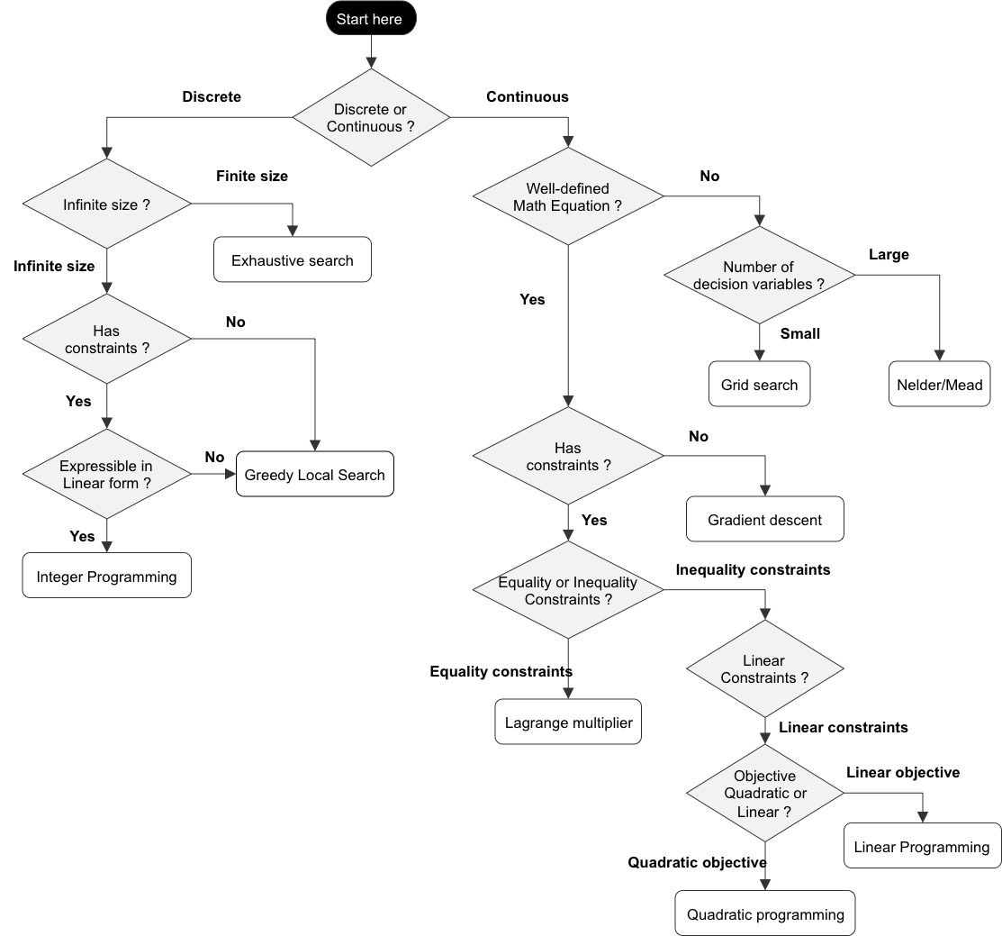
Once we formulate the dependency function, depends on the format of these function, we can employ different optimization methods.  Here is how I choose the appropriate method based on the formulation of dependency functions.

Additional Challenges

To summarize, we have following the process below

1. Define an objective function, constraints, decision variables and environment variables
2. Identify the relationship between different variables
3. Collect or predict those environment variables
4. Optimize those decision variables based on the objective functions
5. Return the optimal value of decision variables as the answer

So far, our dependency graph is acyclic where our decision won't affect the underlying variables.  Although this is reasonably true if the enterprise is an insignificant small player in the market, it is no longer true if the enterprise is one of the few major players.  For example, their pricing strategy may causes other competitors to change their own pricing strategy as well.  And how the competitors would react is less predictable and historical data play a less important role here.  At some point, human judgement will get involved to fill the gaps.

Diverse recommender

This is a continuation of my previous blog in recommendation systems, which describes some basic algorithm for building recommendation systems.  These techniques evaluate each item against user's interest independently and pick the topK items to construct the recommendation.  However, it suffers from the lack of diversity.  For example, the list may contain the same book with soft cover, hard cover, and Kindle version.  Since human's interests are usually diverse, a better recommendation list should contain items that covers a broad spectrum of user's interests, even though each element by itself is not the most aligned with the user's interests.

In this post, I will discuss a recommendation algorithm that consider diversity in its list of recommendation.

Topic Space

First of all, lets define a "topic space" where both the content and user will be map to.  Having a "topic space" is a common approach in recommendation because it can reduce dimensionality and resulting in better system performance and improved generality.

The set of topics in topic space can be extracted algorithmically using Text Mining techniques such as LDA, but for simplicity here we use a manual approach to define the topic space (topics should be orthogonal to each other, as highly correlated topics can distort the measures).  Lets say we have the following topics defined ...

• Romance
• Sports
• Politics
• Weather
• Horror
• ...

Content as Vector of topic weights

Once the topic space is defined, content author can assign topic weights to each content.  For example, movie can be assigned with genres and web page can be assigned with topics as well.  Notice that a single content can be assigned with multiple topics of different weights.  In other words, each content can be described as a vector of topic weights.

User as Vector of topic weights

On the other hand, user can also be represented as a vector of topic weights based on their interaction of content, such as viewing a movie, visiting a web page, buying a product ... etc.  Such interaction can have a positive or negative effect depends on whether the user like or dislike the content.  If the user like the content, the user vector will have the corresponding topic weight associated with the content increases by multiplying alpha (alpha > 1).  If the user dislike the content, the corresponding topic weight will be divided by alpha.  After each update, the user vector will be normalized to a unit vector.

Diversifying the recommendation

We use a utility function to model the diversity of the document and then maximize the utility function.

 










In practice, A is not computed from the full set of documents, which is usually huge.  The full set of documents is typically indexed using some kind of Inverted index technologies using the set of topics as keywords, each c[j,k] is represented as tf-idf.

User is represented as a "query", and will be sent to the inverted index as a search request.  Relevant documents (based on cosine distance measures w.r.t. user) will be return as candidate set D (e.g. top 200 relevant content).

To pick the optimal set of A out of D, we use a greedy approach as follows ...

1. Start with an empty set A
2. Repeat until |A| > H

• Pick a doc i from D such that by adding it to the set A will maximize the utility function
• Add doc i into A and remove doc i from D

Exploration and Exploitation

"Cold Start" is a common problem happens quite frequent in recommendation system.  When a new item enters, there is no prior history that the recommendation system can use.  Since recommendation is an optimization engine which recommends item that matches the best with the user's interests.  Without prior statistics, the new item will hardly be picked up as recommendation and hence continuously lacking the necessary statistics that the recommendation system can use.

One example is movie recommendation where a movie site recommends movies to users based on their past viewing history.  When a new movie arrives the market, there isn't enough viewing statistics about the movie and therefore the new movie will not have a strong match score and won't be picked as a recommendation.  Because we never learn from those that we haven't recommended, the new movies will continuously not have any statistics and therefore will never be picked in future recommendations.

Another cold start example is online Ad serving when a new Ad enters the Ad repository.

Multilevel Granularity Prediction

One solution of cold-start problem is to leverage existing items that are "SIMILAR" to the new item; "similarity" is based on content attributes (e.g. actors, genres).  Notice that here we are using a coarser level of granularity (group of similar items) for prediction, which can be less accurate than a fine-grain model that use view statistics history for prediction.

In other words, we can make recommendation based on two models of different granularity.  Fine-grain model based on instance-specific history data is preferred because it usually has higher accuracy.  For cold-start problem when the new items don't have history data available, we will fall back to use the coarse-grain model based on other similar items to predict user's interests on the new items.

A common approach is to combine both models of different granularity using different weights where the weights depends on the confidence level of the fine-grain model.  For new items, the fine-grain model will have low confidence and therefore it gives more weights to the coarse-grain model.

However, in case we don't have a coarser level of granularity, or the coarse level is too coarse and doesn't give good prediction.  We have to use the fine-grain model to predict.  But how can we build up the instance-specific history for the fine-grain model when we are not sure if the new items are good recommendation for the user ?

Optimization under Uncertainty

 The core of our problem is we need to optimize under uncertainties.  We have two approaches

1. Exploitation: Make the most optimal choice based on current data.  Because of uncertainty (high variation) the current data may deviate from its true expected value, we may end up picking a non-optimal choice.
2. Exploration: Make a random choice or choices that we haven't made before.  The goal is to gather more data point and reduce the uncertainty.  This may waste our cycles of picking the optimal choice. 

 Lets start with a simple, multi-bandit problem.  There are multiple bandit in a Casino, each Bandit has a different probability to win.  If you know the true underlying winning probability of each bandit, you will pick the one with the highest winning probability and keep playing on that one.
Unfortunately, you don't know the underlying probability and has only a limited number of rounds to play.  How would you choose which bandit to play to maximize the total number of rounds you win.

Our strategy should strike a good balance between exploiting and exploring.  To measure how good the strategy is, there is a concept of "regret", which is the ratio of the two elements

• Value you obtain by following Batch Optimal strategy (after you have done batch analysis and have a clear picture in the underlying probability distribution)
• Value you obtain by following the strategy

We'll pick our strategy to do more Exploration initially when you have a lot of uncertainty, and gradually tune down the ratio of Exploration (and leverage more on Exploitation) as we collected more statistics.

Epsilon-Greedy Strategy 

In the "epsilon-greedy" strategy, at every play we throw a dice between explore and exploit.
With probability p(t) = k/t (where k is a constant and t is the number of tries so far),we pick a bandit randomly with equal chance (regardless of whether the bandit has been picked in the past).  And with probability 1 - p(t), we pick the bandit that has the highest probability of win based on passed statistics.

Epsilon-greedy has the desirable property of spending more time to explore initially and gradually reduce the portion as time passes.  However, it doesn't have a smooth transition between explore and exploit.  Also while it explores, it picks each bandit uniformly without giving more weight to the unexplored bandits.  While it exploits, it doesn't consider the confidence of probability estimation.

Upper Confidence Bound: UCB

In the more sophisticated UCB strategy, each bandit is associated with an estimated mean with a confidence interval.  In every play, we choose the bandit whose upper confidence bound (ie: mean + standard deviation) is the largest.

Initially each bandit has a zero mean and a large confidence interval.  As time goes, we estimated the mean p[i] of bandit i based on how many time it wins since we play the bandit i.  We also adjust the confidence interval (reducing deviation) as we play the bandit.
e.g. standard deviation is (p.(1-p)/n)^0.5

Notice that  the UCB model can be used in a more general online machine learning setting.  We require the machine learning model be able to output its estimation based on a confidence parameter.  As a concrete example, lets say a user is visiting our movie site and we want to recommend a movie to the user, based on a bunch of input features (e.g. user feature, query feature ... etc.).

We can do a first round selection (based on information retrieval technique) to identify movie candidate based on relevancy (ie: user's viewing history or user search query).  For each movie candidate, we can invoke the ML model to estimated interest level, as well as the 68% confidence boundary (the confidence level is arbitrary and need to be hand-tuned, 68% is roughly one standard deviation of a Gaussian distribution).  We then combine them by add the 68% confidence range as an offset to its estimation and recommend the movie that has the highest resulting value.

After recommendation, we monitor whether user click on it, view it ... etc. and the response will be fed back to our ML model as a new training data.  Our ML model is an online learning setting and will update the model with this new training data.  Over time the 68% confidence range will be reduced over time as more and more data is gathered.

Relationship with A/B Testing

For most web sites, we run experiments continuously to improve user experience by trying out different layouts, or to improve user's engagement by recommending different types of contents, or by trying out different things.  In general, we have an objective function that defines what aspects we are trying to optimize, and we run different experiments through A/B testing to try out different combinations of configuration to see which one will maximize our objective function.

When the number of experiments (combinations of different configuration) is small, then A/B is exploration mainly.  In a typical setting, we use the old user experience as a control experiment and use the new user experience as a treatment.  The goal is to test if the treatment causes any significant improvement from the control.  Certain percentage of production users (typically 5 - 10%) will be directed to the new experience and we measured whether the user engagement level (say this is our objective function) has increased significantly in a statistical sense.  Such splitting is typically done by hashing the user id (or browser cookies), and based on the range of the hash code falls to determine whether the user should get the new experience.  This hashing is consistent (same user will hash into the same bucket in subsequent request) and so the user will get the whole new user experience when visiting the web site.

When the number of experiments is large and new experiments comes out dynamically and unpredictable, traditional A/B testing model described above will not be able to keep track of all pairs of control and treatment combination.  In the case, we need to use the dynamic exploration/exploitation mechanism to find out the best user experience.

Using the UCB approach, we can treat each user experience as a bandit that the A/B test framework can choose from.  Throughout the process, A/B test framework will explore/exploit among different user experience to optimize for the objective function.  At any time, we can query the A/B testing framework to find out the latest statistics of each user experience.  This provides a much better way to look at large number of experiment result at the same time.

Six steps in data science

"Data science" and "Big data" has become a very hot term in last 2 years.  Since the data storage price dropped significantly, enterprises and web companies has collected huge amount of their customer's behavioral data even before figuring out how to use them.  Enterprises also start realizing that these data, if use appropriately, can turn into useful insight that can guide its business along a more successful path.

From my observation, the effort of data science can be categorized roughly into the following areas.

• Data acquisition
• Data visualization
• OLAP, Report generation
• Response automation
• Predictive analytics
• Decision optimization

Data Acquisition

Data acquisition is about collecting data into the system.  This is an important step before any meaningful processing or analysis can begin.  Most companies start with collecting business transaction records from their OLTP system.  Typically there is an ETL (Extract/Transform/Load) process involved to ingest the raw data, clean the data and transform them appropriately.  Finally, the data is loaded into a data warehouse where the subsequent data analytics exercises are performed.  In today's big data world, the destination has been shifted from traditional data warehouse to Hadoop distributed file system (HDFS).

Data Visualization

Data visualization is usually the first step of analyzing the data.  It is typically done by plotting data in different ways to establish give a quick sense of its shape, in order to guide the data scientist to determine what subsequent analysis should be conducted.  This is also where a more experience data scientist can be distinguished from an less experienced one based on how fast they can spot common patterns or anomalies from data.  Most of the plotting package works only for data that fits into one single machine.  Therefore, in the big data world, data sampling is typically conducted first to reduce the data size, and then import to a single machine where R, SAS, SPSS can be used to visualized the sample data.

OLAP / Reporting

OLAP is about aggregating transaction data (e.g. revenue) along different dimensions (e.g. Month, Location, Product) where the enterprise defines its KPI/business metrics that measures the companies' performance.  This can be done either in an ad/hoc manner (OLAP), or in a predefined manner (Report template).  Report writer (e.g. Tableau, Microstrategy) are use to produce the reports.  The data is typically stored in regular RDBMS or a multidimensional cube which is optimizing for OLAP processing (ie: slice, dice, rollup, drilldown).  In the big data world, Hive provides a SQL-like access mechanism and is commonly used to access data stored in HDFS.  Most popular report writers have integrated with Hive (or declare plan to integrate with it) to access big data stored in HDFS.

Response Automation

Response automation is about leveraging domain-specific knowledge to encode a set of "rules" which include event/condition/action.  The system monitors all events observed, matches them against the conditions, (which can be a boolean expression of event attributes, or a sequence of event occurrence), and trigger appropriate actions.  In the big data world, automating such response is typically done by stream processing mechanism (such as Flume and Storm).  Notice that the "rule" need to be well-defined and unambiguous.

Predictive Analytics

Prediction is about estimating unknown data based on observed data through statistical/probabilistic approach.  Depends on the data type of the output, "prediction" can be subdivided into "classification" (when the output is a category) or "regression" (when the output is a number).

Prediction is typically done by first "train" a predictive model using historic data (where all input and output value is known).  This training is done via an iterative process where the performance of the model in each iteration is measured at the end of each iteration.  Additional input data or different model parameters will be used in next round of iteration.  When the predictive performance is good enough and no significant improvement is made between subsequent iterations, the process will stop and the best model created during the process will be used.

Once we have the predictive model, we can use it to predict information we haven't observed, either this is information that is hidden, or hasn't happen yet (ie: predicting future)

For a more detail description of what is involved in performing predictive analytics, please refer to my following blog.

• Overview and Data visualization
• Data Preparation
• Generalized Linear Regression
• NeuralNet, Bayesian, SVM, KNN
• Decision Tree and Ensembles
• Evaluate Model Performance

Decision Optimization

Decision optimization is about making the best decision after carefully evaluating possible options against some measure of business objectives.  The business objective is defined by some "objective function" which is expressed as a mathematical formula of some "decision variables".  Through various optimization technique, the system will figure out what the decision variables should be in order ro maximize (or minimize) the value of the objective function.  The optimizing technique for discrete decision variables is typically done using exhaustive search, greedy/heuristic search, integer programming technique, while optimization for continuous decision variables is done using linear/quadratic programming.

From my observation, "decision optimization" is the end goal of most data science effort.  But "decision optimization" relies on previous effort.  To obtain the overall picture (not just observed data, but also hidden or future data) at the optimization phase, we need to make use of the output of the prediction.  And in order to train a good predictive model, we need to have the data acquisition to provide clean data.  All these efforts are inter-linked with each other in some sense.