Machine Learning in R: Clustering

Clustering is a very common technique in unsupervised machine learning to discover groups of data that are "close-by" to each other. It is broadly used in customer segmentation and outlier detection.

It is based on some notion of "distance" (the inverse of similarity) between data points and use that to identify data points that are close-by to each other. In the following, we discuss some very basic algorithms to come up with clusters, and use R as examples.

K-Means
This is the most basic algorithm

1. Pick an initial set of K centroids (this can be random or any other means)
2. For each data point, assign it to the member of the closest centroid according to the given distance function
3. Adjust the centroid position as the mean of all its assigned member data points. Go back to (2) until the membership isn't change and centroid position is stable.
4. Output the centroids.

Notice that in K-Means, we not only require the distance function to be defined but also requiring the mean function to be specified as well. Of course, we also need K (the number of centroids) to be specified.

K-Means is highly scalable with O(n * k * r) where r is the number of rounds, which is a constant depends on the initial pick of centroids. Also notice that the result of each round is undeterministic. The usual practices is to run multiple rounds of K-Means and pick the result of the best round. The best round is one who minimize the average distance of each point to its assigned centroid.

Here is an example of doing K-Means in R

> km <- kmeans(iris[,1:4], 3)
> plot(iris[,1], iris[,2], col=km$cluster)
> points(km$centers[,c(1,2)], col=1:3, pch=8, cex=2)
> table(km$cluster, iris$Species)

setosa versicolor virginica
1      0         48        14
2     50          0         0
3      0          2        36

with the following visual output.

Hierarchical Clustering
In this approach, it compares all pairs of data points and merge the one with the closest distance.

1. Compute distance between every pairs of point/cluster. Compute distance between pointA to pointB is just the distance function. Compute distance between pointA to clusterB may involve many choices (such as the min/max/avg distance between the pointA and points in the clusterB). Compute distance between clusterA to clusterB may first compute distance of all points pairs (one from clusterA and the other from clusterB) and then pick either min/max/avg of these pairs.
2. Combine the two closest point/cluster into a cluster. Go back to (1) until only one big cluster remains.

In hierarchical clustering, the complexity is O(n^2), the output will be a Tree of merge steps. It doesn't require us to specify K or a mean function. Since its high complexity, hierarchical clustering is typically used when the number of points are not too high.

Here is an example of doing hierarchical clustering in R

> sampleiris <- iris[sample(1:150, 40),]
> distance <- dist(sampleiris[,-5], method="euclidean")
> cluster <- hclust(distance, method="average")
> plot(cluster, hang=-1, label=sampleiris$Species)

with the following visual output

Fuzzy C-Means
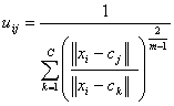
Unlike K-Means where each data point belongs to only one cluster, in fuzzy cmeans, each data point has a fraction of membership to each cluster. The goal is to figure out the membership fraction that minimize the expected distance to each centroid.

The algorithm is very similar to K-Means, except that a matrix (row is each data point, column is each centroid, and each cell is the degree of membership) is used.

1. Initialize the membership matrix U
2. Repeat step (3), (4) until converge
3. Compute location of each centroid based on the weighted fraction of its member data point's location.
4. Update each cell as follows

Notice that the parameter m is the degree of fuzziness. The output is the matrix with each data point assigned a degree of membership to each centroids.
Here is an example of doing Fuzzy c-means in R

> library(e1071)
> result <- cmeans(iris[,-5], 3, 100, m=2, method="cmeans")
> plot(iris[,1], iris[,2], col=result$cluster)
> points(result$centers[,c(1,2)], col=1:3, pch=8, cex=2)
> result$membership[1:3,]
         1           2         3
[1,] 0.001072018 0.002304389 0.9966236
[2,] 0.007498458 0.016651044 0.9758505
[3,] 0.006414909 0.013760502 0.9798246
> table(iris$Species, result$cluster)
        1  2  3
setosa      0  0 50
versicolor  3 47  0
virginica  37 13  0

with the following visual output (very similar to K-Means)

Multi-Gaussian with Expectation-Maximization
Generally in machine learning, we will to learn a set of parameters that maximize the likelihood of observing our training data. However, what if there are some hidden variable in our data that we haven't observed. Expectation Maximization is a very common technique to use the parameter to estimate the probability distribution of those hidden variable, compute the expected likelihood and then figure out the parameters that will maximize this expected likelihood. It can be explained as follows ...

Now, we assume the underlying data distribution is based on K centroids, each a multi-variate Gaussian distribution. To map Expectation / Maximization into this, we have the following.

The order of complexity is similar to K-Means with a larger constant. It also requires K to be specified. Unlike K-Means whose cluster is always in circular shape. Multi-Gaussian can discover cluster with elliptical shape with different orientation and hence it is more general than K-Means.

Here is an example of doing multi-Gaussian with EM in R

> library(mclust)
> mc <- Mclust(iris[,1:4], 3)
> plot(mc, data=iris[,1:4], what=c('classification'),
       dimens=c(3,4))
> table(iris$Species, mc$classification)

 1  2  3
setosa     50  0  0
versicolor  0 45  5
virginica   0  0 50

with the following visual output

Density-based Cluster
In density based cluster, a cluster is extend along the density distribution. Two parameters is important: "eps" defines the radius of neighborhood of each point, and "minpts" is the number of neighbors within my "eps" radius. The basic algorithm called DBscan proceeds as follows

1. First scan: For each point, compute the distance with all other points. Increment a neighbor count if it is smaller than "eps".
2. Second scan: For each point, mark it as a core point if its neighbor count is greater than "minpts"
3. Third scan: For each core point, if it is not already assigned a cluster, create a new cluster and assign that to this core point as well as all of its neighbors within "eps" radius.

Unlike other cluster, density based cluster can have some outliers (data points that doesn't belong to any clusters). On the other hand, it can detect cluster of arbitrary shapes (doesn't have to be circular at all)

Here is an example of doing DBscan in R

> library(fpc)
# eps is radius of neighborhood, MinPts is no of neighbors
# within eps
> cluster <- dbscan(sampleiris[,-5], eps=0.6, MinPts=4)
> plot(cluster, sampleiris)
> plot(cluster, sampleiris[,c(1,4)])
# Notice points in cluster 0 are unassigned outliers
> table(cluster$cluster, sampleiris$Species)

setosa versicolor virginica
0      1          2         6
1      0         13         0
2     12          0         0
3      0          0         6

with the following visual output ... (notice the black points are outliers, triangles are core points and circles are boundary points)

Although this has covered a couple ways of finding cluster, it is not an exhaustive list. Also here I tried to illustrate the basic idea and use R as an example. For really large data set, we may need to run the clustering algorithm in parallel. Here is my earlier blog about how to do K-Means using Map/Reduce as well as Canopy clustering as well.

K-Means Clustering in Map Reduce

Unsupervised machine learning has broad application in many e-commerce sites and one common usage is to find clusters of consumers with common behaviors. In clustering methods, K-means is the most basic and also efficient one.

K-Means clustering involve the following logical steps

1) Determine the value of k
2) Determine the initial k centroids
3) Repeat until converge
- Determine membership: Assign each point to the closest centroid
- Update centroid position: Compute new centroid position from assigned members

Determine the value of K
This is basically asking the question of: "How many clusters you are interested to discover ?"
So the answer is specific to the problem domain.

One way is to try different K. At some point, we'll see increasing K doesn't help much to improve the overall quality of clustering. Then that is the right value of K.

Notice that the overall quality of cluster is the average distance from each data point to its associated cluster.


Determine the initial K centroids
We need to pick K centroids to start the algorithm. So one way to pick them is to randomly pick K points from the whole data set.

However, picking a good set of centroids can reduce the number of subsequent iterations and by "good" I mean the K centroid should be as far apart to each other as possible, or even better the initial K centroid is close to the final K centroid. As you can see, choosing the random K points is reasonable but non-optimum.

Another approach is to take a small random sample set from the input data set and do a hierarchical clustering within this smaller set (note that hierarchical clustering is not-scaling to large data set).

We can also partition the space into overlapping region using canopy cluster technique (describe below) and pick the center of each canopy as the initial centroid.

Iteration
Each iteration is implemented as a Map/Reduce job. First of all, we need a control program on the client side to initialize the centroid positions, kickoff the iteration of Map/Reduce jobs and determine whether the iteration should end ...

kmeans(data) {
  initial_centroids = pick(k, data)
  upload(data)
  writeToS3(initial_centroids)
  old_centroids = initial_centroids
  while (true){
    map_reduce()
    new_centroids = readFromS3()
    if change(new_centroids, old_centroids) < delta {
      break
    } else {
      old_centroids = new_centroids
    }
  }
  result = readFromS3()
  return result
}

Within each iteration, most of the processing will be done in the Map task, which determine the membership for each point, as well as compute a partial sum of each member points of each cluster.

The reducer did the easy job by aggregating all partial sums and compute the update centroid position, and then out them into a shared store (S3 in this case) that can be picked up by the Map/Reduce job of next round.



Complexity Analysis
Most of the work is done by the Mapper and the workload is pretty balanced. So the time complexity will be O(k*n/p) where k is number of clusters, n is number of data points and p is number of machines. Note that the factor of k comes in at the closest_centroid() function above when comparing each data point with each intermediate centroid as follows ...

closest_centroid(point, listOfCentroids) {
  bestCentroid = listOfCentroids[0]
  minDistance = INFINITY
  for each centroid in listOfCentroids {
    distance = dist(point, centroid)
    if distance < minDistance {
      minDistance = distance
      bestCentroid = centroid
    }
  }
  return bestCentroid
}

If we partition the space into proximity regions, we only need to compare each point with centroid within the same proximity region and treat other centroids infinite distance. In other words, we don't have to compare each point with all k centroids.

Canopy clustering provide such a partitioning mechanism.


Canopy Clustering
To define the proximity region (canopy), we can draw a circle (or hypersphere) centered at a data point. Points outside this sphere is considered to be too far.

However, if we apply this definition to every point, then we will have as many proximity region as the number of points, which ends up doesn't save much processing. We also observed that points are very close by each other can stay in the same region without each point creating their own. Therefore, we can draw a smaller circle within the big circle (with the same center) such that data points within the small circle is not allowed to form its own proximity region.


Notice that each proximity region can overlap with each other and the degree of overlapping will be affected by the choice of T1. Also the choice of T2 affects how many canopies will be formed. Picking the right number of T1 and T2 is domain-specific, and also depends on the number of clusters and the space volume. If there is a small number of clusters within a big space, then a bigger T1 should be chosen.

To create the canopies (and mark the data points with the canopies), we will do the following steps ...
1) Create the canopy centers, with one scan

• Keep a list of canopies, initially an empty list
• Scan each data point, if it is within T2 distance of existing canopies, discard it. Otherwise, add this point into the list of canopies

2) Assign data points to the canopies, with another scan

• Start with a list of canopies from last step
• Scan each data point, if it is within T1 of the canopyA, add A as the assigned canopy to the data point. Notice that the data point can be assigned to multiple canopies
• When done, each data point will look like
  

Notice that now the input data points has been added with an extra attribute that contains the assigned canopies. When compare the point with the intermediate centroids, we only need to compare centroids within the same canopy. Here is the modified version of the algorithm ...

closest_centroid(point, listOfCentroids) {
  bestCentroid = listOfCentroids[0]
  minDistance = INFINITY
  for each cent in listOfCentroids {
    if (not point.myCanopy.intersects(cent.myCanopy)) {
      continue
    }
    distance = dist(point, centroid)
    if distance < minDistance {
      minDistance = distance
      bestCentroid = centroid
    }
  }
  return bestCentroid
}